Excel Visual Basic for Applications Tutorial
Introduction
Excel Visual Basic for Applications is a very useful tool if one deals with Excel on a daily basis. One can automate Excel commands using Visual Basic for Applications (VBA) such that tedious tasks can be done with a click of a button. VBA can also be very useful if one deals with data and needs to present it in a clear manner.
Adding the Developer Tab
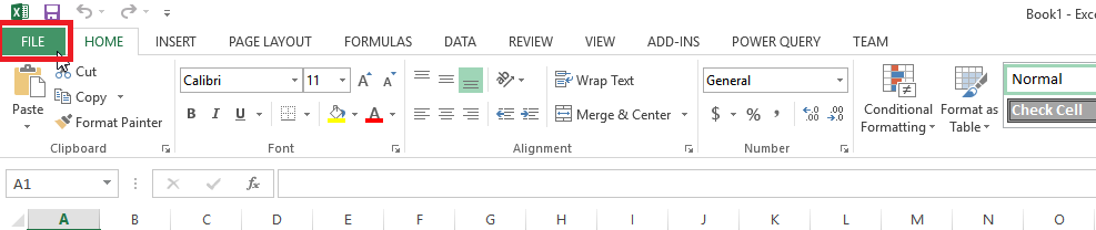
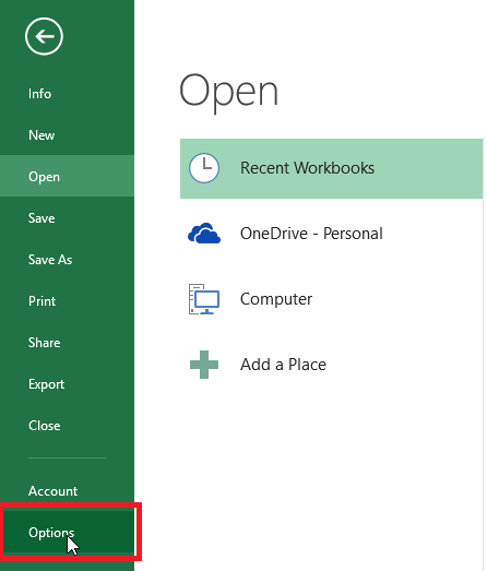
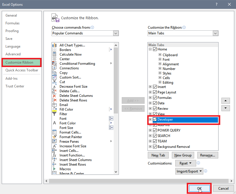
The first step in creating Excel VBA Macros is to add the Developer tab on the Ribbon. Select File in the upper-left corner of the Excel Menu and then select Options. Select Customize Ribbon and enable the Developer option under Main Tabs.
File
Options
Customize Ribbon
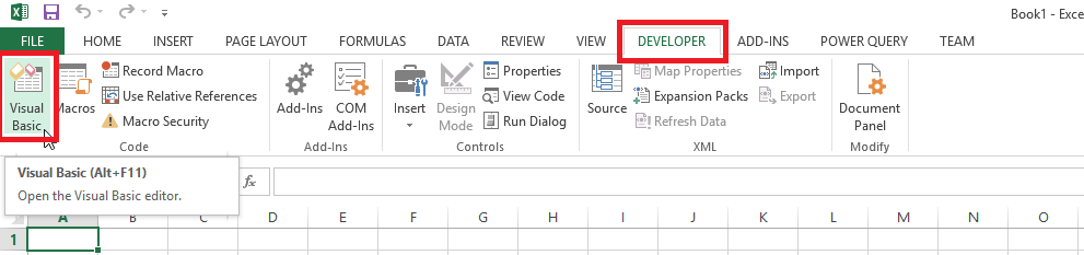
You should now see the Developer tab on your Ribbon. Select the Visual Basic option to open up the editor.
Developer Tab
A new window will pop up where you can select Module from the dropdown menu next to the Save icon.
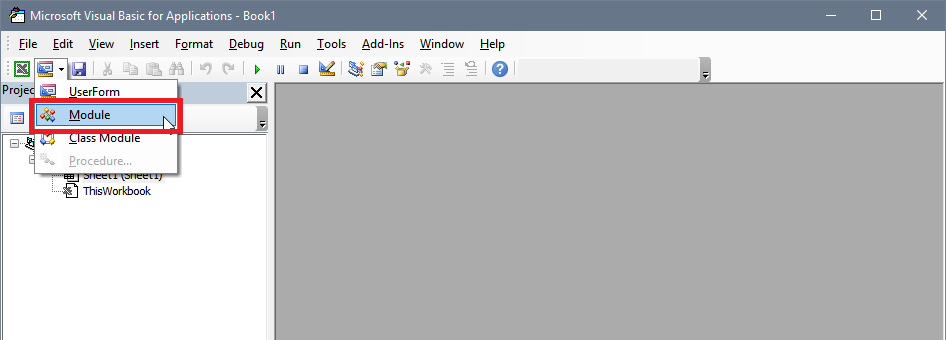
Create Module
You can now start creating subroutines in VBA by typing sub SUBNAME in the editor window. Hitting enter right after your subroutine's name should automatically fill in the parentheses and the End Sub text. All your code will be within Sub SUBNAME() and End Sub. The subroutine can be executed by pressing F5 or by selecting the small green arrow.
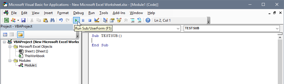
Create Subroutine
One last step must be done before we continue. Make sure to save the Excel file as an Excel Macro-Enabled Workbook (.xlsm) in order to be able to run the Excel VBA Macros on that workbook.

Excel Macro-Enabled Workbook (.xlsm)
Cells
The cells in Excel are what contain the information and data of the workbook. Being able to modify these cells is very important if one wants to automate tasks efficiently. This section will be dedicated to cells and how one can modify them.
Clear Cells
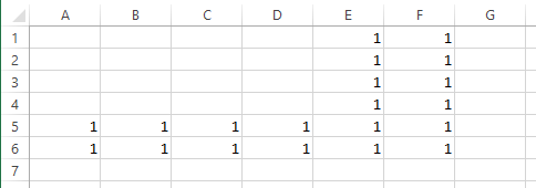
Cells can be assigned values several different ways but it is also important to know how to clear the contents of a cell if we want to clean up the worksheet in order to test out new code. The command .ClearContents clears the contents of the specified cells. The first command below clears the contents of Cell(1,1), the second command clears the contents of the Range(Cells(1, 1), Cells(4, 4)), and the last command clears the contents of the whole worksheet.
Input:Cells(1, 1).ClearContents
Clear Contents
Output:
Cell(1,1) Clear Contents
Input:
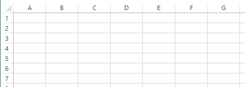
Range(Cells(1, 1), Cells(4, 4)).ClearContents
Output:
Range(Cells(1, 1), Cells(4, 4)) Clear Contents
Input:
Cells.ClearContents
Output:
Clear All Contents
Assigning Values to Cells
One can assign values to cells by using the Cells(ROW,COLUMN) command. Here we assign values to cells directly or through variables. A cell can be assigned a string using quotation ("") marks.
Input:Cells(1, 3) = 1
Cells(3, 1) = "Test"
Var1 = 5.5
Cells(6, 5) = Var1
Var2 = "Test2"
Cells(5, 6) = Var2
Output:
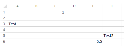
Cells Output
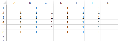
You can also use the range command to assign values to one cell or multiple cells. The range starts at the top left corner and covers everything down to the bottom right corner of the given values.
Input:Range("A1") = 1
Output:
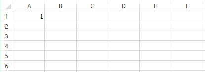
Range A1
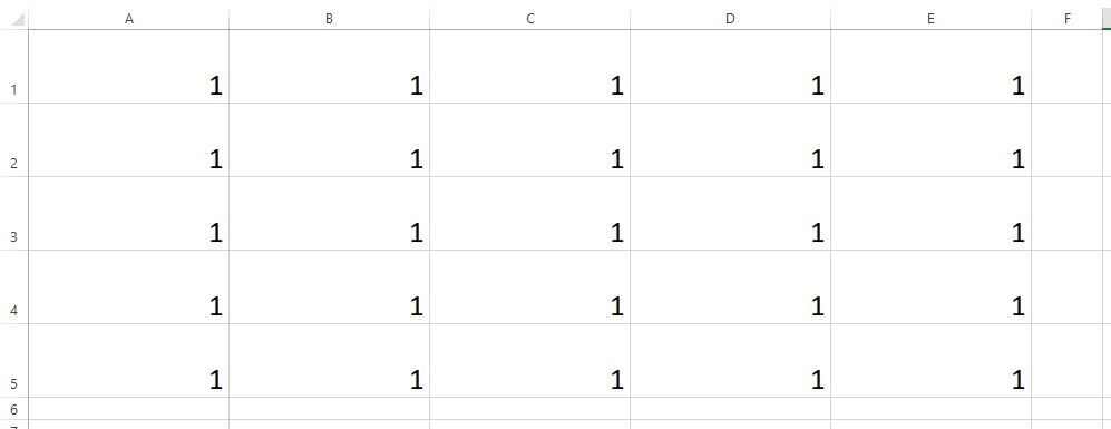
Input:
Range("A1:E5") = 1
Output:
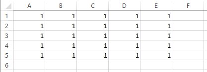
Range A1:E5
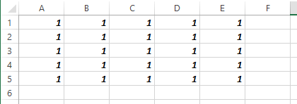
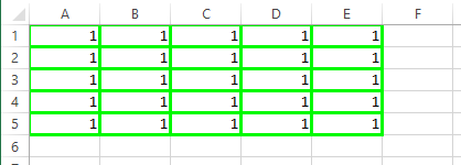
The cells command can also be used within the range command.
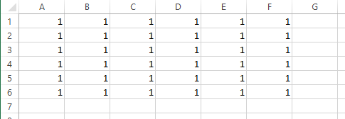
Input:Range(Cells(1, 1), Cells(5, 5)) = 1
Output:
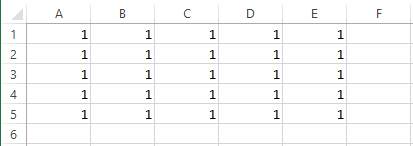
Range Cells A1:E5
Variables can be used to enter the desired cell locations which is very convenient when dealing with dynamic data ranges. The LastRow and LastColumn variables have both been assigned a value of 3 in this example but the Last Row and Last Column section introduces a very useful method on finding the exact last row and last column of a data range dynamically.
Input:LastRow = 3
LastColumn = 3
Range(Cells(1, 1), Cells(LastRow, LastColumn)) = 1
Output:
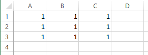
Range LastRow LastColumn
A combination of cells and ranges can be used to assign values to cells as well. The range command below is mimicking Range("A1:D4") = 1 by using the & symbol to concatenate strings and numbers. Strings can be concatenated using the & symbol as well. Notice the space in the quotation marks for Cells(6, 6) and Cells(7, 7) in order to create a space in the actual cell entry.
Input:FirstRow = 1
LastRow = 4
Range("A" & FirstRow & ":D" & LastRow) = 1
Cells(5, 5) = "Test" & 5
Cells(6, 6) = "Another " & "Test"
Cells(7, 7) = "Another" & " Test"
Output:
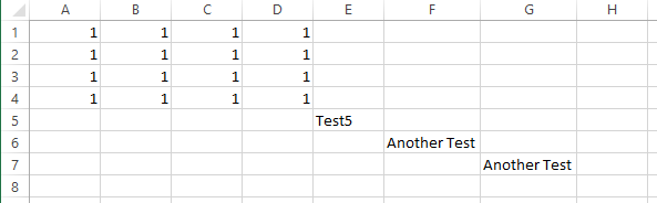
Range Combination
Customize Cells
One of Excel's greatest features is the possibility to customize your data and display it in an eye-catching manner. Excel VBA can also be used to customize cells in many different ways. Before we continue, the code below erases the contents (.ClearContents), erases the formatting (.ClearFormats), and reverts the row height (RowHeight = 15) and column width (.ColumnWidth = 8.43) back to default for all cells. This will be useful when we want to clear a sheet in order to run new code.
Input:Cells.ClearContents
Cells.ClearFormats
Cells.RowHeight = 15
Cells.ColumnWidth = 8.43
Clear Contents
Output:
Default
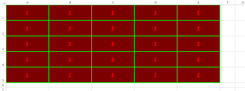
The .Interior.Color command changes the color of the specified cells. The code below uses the RGB format to select the desired color.
Input:LastRow = 5
LastColumn = 5
Range(Cells(1, 1), Cells(LastRow, LastColumn)) = 1
Range(Cells(1, 1), Cells(LastRow, LastColumn)).Interior.Color = RGB(125, 0, 0)
Output:
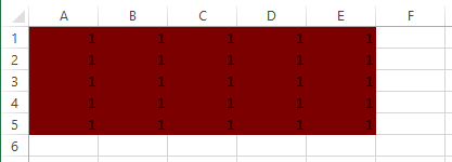
Interior Color
You can acquire the numbers for the RGB colors by selecting the Home tab and clicking on More Colors under the paint bucket icon. You can now select one of the default colors in the Standard tab then click on the Custom tab in order to get the RGB color numbers. You can also customize your own color with the Custom tab.
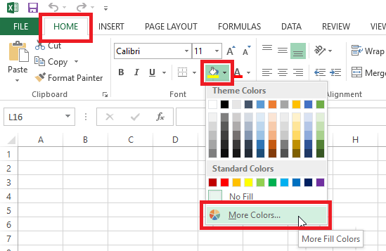
More Colors
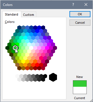
Standard Colors
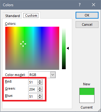
Custom Colors
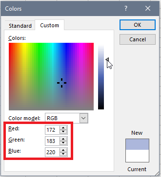
Customize Custom Colors
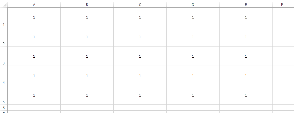
The .Font.Color command changes the color of the font for the specified cells.
Input:LastRow = 5
LastColumn = 5
Range(Cells(1, 1), Cells(LastRow, LastColumn)) = 1
Range(Cells(1, 1), Cells(LastRow, LastColumn)).Font.Color = RGB(250, 0, 0)
Output:
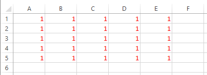
Font Color
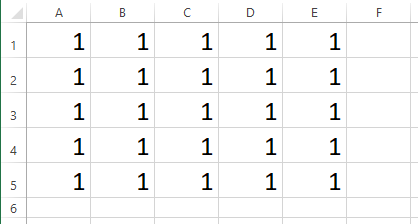
The .Font.Size command changes the font size for the specified cells.
Input:LastRow = 5
LastColumn = 5
Range(Cells(1, 1), Cells(LastRow, LastColumn)) = 1
Range(Cells(1, 1), Cells(LastRow, LastColumn)).Font.Size = 20
Output:
Font Size
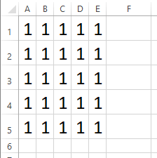
Changing the font size of a cell can lead to the contents of the cell to be obscured by the cell's default row height and column width. The .AutoFit command can be used for both the Rows and Columns of a range in order to automatically adjust the height and width, respectively, of a cell to the size of the cell's contents.
Input:LastRow = 5
LastColumn = 5
Range(Cells(1, 1), Cells(LastRow, LastColumn)) = 1
Range(Cells(1, 1), Cells(LastRow, LastColumn)).Font.Size = 20
Range(Cells(1, 1), Cells(LastRow, LastColumn)).Rows.AutoFit
Output:
Rows Auto Fit
Input:
LastRow = 5
								LastColumn = 5
								Range(Cells(1, 1), Cells(LastRow, LastColumn)) = 1

								Range(Cells(1, 1), Cells(LastRow, LastColumn)).Font.Size = 20
Range(Cells(1, 1), Cells(LastRow, LastColumn)).Columns.AutoFit
Output:
Columns Auto Fit
Input:
LastRow = 5
								LastColumn = 5
								Range(Cells(1, 1), Cells(LastRow, LastColumn)) = 1
								Range(Cells(1, 1), Cells(LastRow, LastColumn)).Font.Size = 20

								Range(Cells(1, 1), Cells(LastRow, LastColumn)).Rows.AutoFit
Range(Cells(1, 1), Cells(LastRow, LastColumn)).Columns.AutoFit
Output:
Rows and Columns Auto Fit
The row height and column width can be manually specified by using the .RowHeight and .ColumnWidth commands, respectively. Note that all the rows and columns of that range adjust accordingly.
Input:LastRow = 5
LastColumn = 5
Range(Cells(1, 1), Cells(LastRow, LastColumn)) = 1
Range(Cells(1, 1), Cells(LastRow, LastColumn)).RowHeight = 50
Range(Cells(1, 1), Cells(LastRow, LastColumn)).ColumnWidth = 25
Output:
Rows and Columns Size
The font can be bolded and italicized using the .Font.Bold = True and .Font.Italic = True commands, respectively.
Input:LastRow = 5
LastColumn = 5
Range(Cells(1, 1), Cells(LastRow, LastColumn)) = 1
Range(Cells(1, 1), Cells(LastRow, LastColumn)).Font.Bold = True
Range(Cells(1, 1), Cells(LastRow, LastColumn)).Font.Italic = True
Output:
Bold and Italic Font
The contents of a cell can be aligned both horizontally and vertically using the .HorizontalAlignment and .VerticalAlignment commands, respectively. Here we are centering the cell both horizontally and vertically using xlCenter. I included the resizing of the rows and columns to better illustrate the alignment of a cell's content.
Input:LastRow = 5
LastColumn = 5
Range(Cells(1, 1), Cells(LastRow, LastColumn)) = 1
Range(Cells(1, 1), Cells(LastRow, LastColumn)).RowHeight = 50
Range(Cells(1, 1), Cells(LastRow, LastColumn)).ColumnWidth = 25
Range(Cells(1, 1), Cells(LastRow, LastColumn)).HorizontalAlignment = xlCenter
Range(Cells(1, 1), Cells(LastRow, LastColumn)).VerticalAlignment = xlCenter
Output:
Alignment
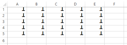
We can create borders for cells in a range by using the .Borders.LineStyle command. The border weight can also be adjusted with the .Borders.Weight command. There are various border styles and weights as seen below.
Input:LastRow = 5
LastColumn = 5
Range(Cells(1, 1), Cells(LastRow, LastColumn)) = 1
Range(Cells(1, 1), Cells(LastRow, LastColumn)).Borders.LineStyle = xlContinuous
Output:
Regular Border
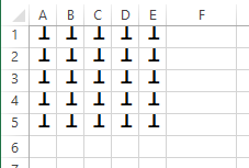
Input:
LastRow = 5
LastColumn = 5
Range(Cells(1, 1), Cells(LastRow, LastColumn)) = 1
Range(Cells(1, 1), Cells(LastRow, LastColumn)).Borders.LineStyle = xlDash
Output:
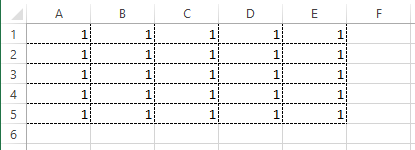
Dash Border
Input:
LastRow = 5
LastColumn = 5
Range(Cells(1, 1), Cells(LastRow, LastColumn)) = 1
Range(Cells(1, 1), Cells(LastRow, LastColumn)).Borders.LineStyle = xlDouble
Output:
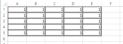
Double Border
Input:
LastRow = 5
								LastColumn = 5
								Range(Cells(1, 1), Cells(LastRow, LastColumn)) = 1

								Range(Cells(1, 1), Cells(LastRow, LastColumn)).Borders.LineStyle = xlContinuous
Range(Cells(1, 1), Cells(LastRow, LastColumn)).Borders.Weight = xlThick
Output:
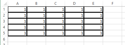
Regular Border Thick
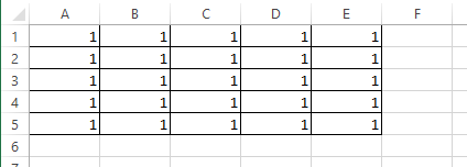
Input:
LastRow = 5
								LastColumn = 5
								Range(Cells(1, 1), Cells(LastRow, LastColumn)) = 1
								Range(Cells(1, 1), Cells(LastRow, LastColumn)).Borders.LineStyle = xlContinuous

								Range(Cells(1, 1), Cells(LastRow, LastColumn)).Borders.Weight = xlThin
Output:
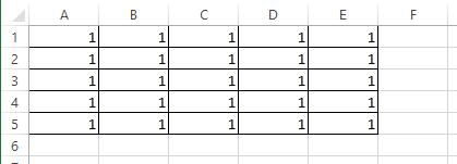
Regular Border Thin
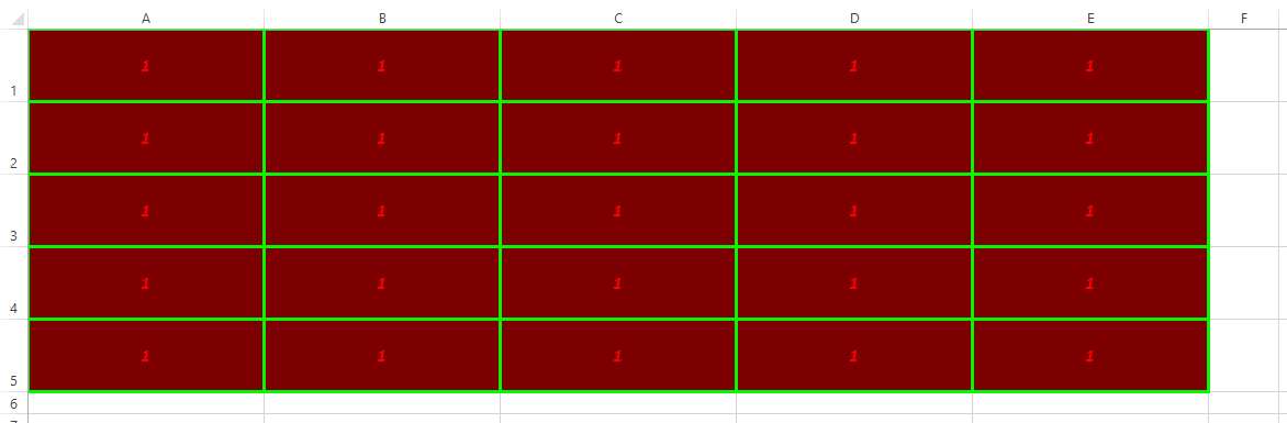
The border color can be changed using the .Borders.Color command.
Input:LastRow = 5
LastColumn = 5
Range(Cells(1, 1), Cells(LastRow, LastColumn)) = 1
Range(Cells(1, 1), Cells(LastRow, LastColumn)).Borders.LineStyle = xlContinuous
Range(Cells(1, 1), Cells(LastRow, LastColumn)).Borders.Weight = xlThick
Range(Cells(1, 1), Cells(LastRow, LastColumn)).Borders.Color = RGB(0, 250, 0)
Output:
Border Color
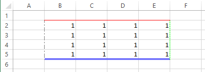
You can also customize specific edges of cells by stating which edge you want to modify within the .Border(xlEdgeSIDE) command. Note that the specified edge side applies to the outer edges of the entire range and not the individual cells. I moved the cells to better illustrate the borders.
Input:LastRow = 5
LastColumn = 5
Range(Cells(2, 2), Cells(LastRow, LastColumn)) = 1
Range(Cells(2, 2), Cells(LastRow, LastColumn)).Borders(xlEdgeTop).LineStyle = xlContinuous
Range(Cells(2, 2), Cells(LastRow, LastColumn)).Borders(xlEdgeRight).LineStyle = xlDash
Range(Cells(2, 2), Cells(LastRow, LastColumn)).Borders(xlEdgeBottom).LineStyle = xlDouble
Range(Cells(2, 2), Cells(LastRow, LastColumn)).Borders(xlEdgeLeft).LineStyle = xlDashDot
Range(Cells(2, 2), Cells(LastRow, LastColumn)).Borders(xlEdgeTop).Color = RGB(250, 0, 0)
Range(Cells(2, 2), Cells(LastRow, LastColumn)).Borders(xlEdgeRight).Color = RGB(0, 250, 0)
Range(Cells(2, 2), Cells(LastRow, LastColumn)).Borders(xlEdgeBottom).Color = RGB(0, 0, 250)
Range(Cells(2, 2), Cells(LastRow, LastColumn)).Borders(xlEdgeLeft).Color = RGB(125, 125, 125)
Output:
Border Color
The style of the cells can be changed using the .Style command. Below are a couple of different style formats.
Input:LastRow = 5
LastColumn = 5
Range(Cells(1, 1), Cells(LastRow, LastColumn)) = 1
Range(Cells(1, 1), Cells(1, LastColumn)).Style = "Currency"
Range(Cells(2, 1), Cells(2, LastColumn)).Style = "Percent"
Range(Cells(3, 1), Cells(3, LastColumn)).Style = "Comma"
Range(Cells(4, 1), Cells(4, LastColumn)).Style = "Good"
Range(Cells(5, 1), Cells(5, LastColumn)).Style = "Bad"
Output:
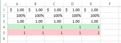
Style Formats
All these different modifications can be combined to create your personal format as seen in the first code below. However, the first code can be written in a more compact manner by using the With command which the second code uses. Anything in the With block will be applied to what is stated right after the With command. In the second code, all the formatting within With is applied to Range(Cells(1, 1), Cells(LastRow, LastColumn)). Both codes result in the same outcome but one is easier to read and more compact than the other.
Input:LastRow = 5
LastColumn = 5
Range(Cells(1, 1), Cells(LastRow, LastColumn)) = 1
Range(Cells(1, 1), Cells(LastRow, LastColumn)).Interior.Color = RGB(125, 0, 0)
Range(Cells(1, 1), Cells(LastRow, LastColumn)).Font.Color = RGB(250, 0, 0)
Range(Cells(1, 1), Cells(LastRow, LastColumn)).Font.Size = 20
Range(Cells(1, 1), Cells(LastRow, LastColumn)).RowHeight = 50
Range(Cells(1, 1), Cells(LastRow, LastColumn)).ColumnWidth = 25
Range(Cells(1, 1), Cells(LastRow, LastColumn)).Font.Bold = True
Range(Cells(1, 1), Cells(LastRow, LastColumn)).Font.Italic = True
Range(Cells(1, 1), Cells(LastRow, LastColumn)).HorizontalAlignment = xlCenter
Range(Cells(1, 1), Cells(LastRow, LastColumn)).VerticalAlignment = xlCenter
Range(Cells(1, 1), Cells(LastRow, LastColumn)).Borders.LineStyle = xlContinuous
Range(Cells(1, 1), Cells(LastRow, LastColumn)).Borders.Weight = xlThick
Range(Cells(1, 1), Cells(LastRow, LastColumn)).Borders.Color = RGB(0, 250, 0)
Output:
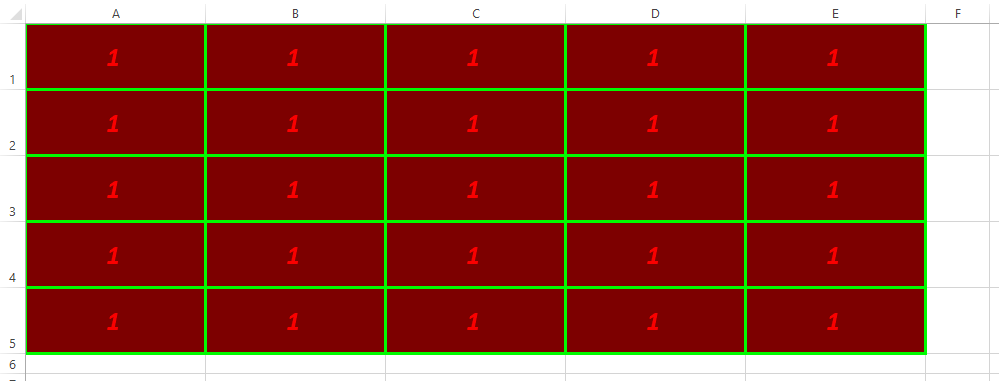
Combined Formats
Input:
LastRow = 5
								LastColumn = 5
								Range(Cells(1, 1), Cells(LastRow, LastColumn)) = 1


								With Range(Cells(1, 1), Cells(LastRow, LastColumn))

								.Interior.Color = RGB(125, 0, 0)

								    .Font.Color = RGB(250, 0, 0)

								    .Font.Size = 20

								    .RowHeight = 50

								    .ColumnWidth = 25

								    .Font.Bold = True
								    .Font.Italic = True

								    .HorizontalAlignment = xlCenter
								    .VerticalAlignment = xlCenter

								    .Borders.LineStyle = xlContinuous

								    .Borders.Weight = xlThick

								    .Borders.Color = RGB(0, 250, 0)

								End With
Output:
Combined Formats With
Sheets
Sheets are very useful when one has to separate large sets of data according to their subjects. This section will be dedicated to Excel VBA commands that are used to modify sheets.
Create Sheet
Creating a new sheet can be done with the sheets.Add command. The .Add(After:=sheets(sheets.Count)) text adds a sheet after the last sheet in the workbook by using the sheets.Count text instead of a specific sheet name. The .Name command gives the new sheet a name, e.g. TESTSHEET. The second code adds a sheet in between two new sheets that I have created (TESTSHEET and TESTSHEET2) by specifying the sheet name TESTSHEET in .Add(After:=sheets("TESTSHEET")).
Input:sheets.Add(After:=sheets(sheets.Count)).Name = "TESTSHEET"

New Sheet
Output:

New Sheet Added
Input:
sheets.Add(After:=sheets("TESTSHEET")).Name = "BETWEENTESTSHEET"

Between Sheet
Output:

Between Sheet Added
Delete Sheet
A sheet can be deleted by using the command sheets("SHEETNAME").Delete. A warning will pop up asking if the user is sure they want to delete the sheet, select Delete to delete the sheet.
Input:sheets("BETWEENTESTSHEET").Delete
Between Sheet
Output:
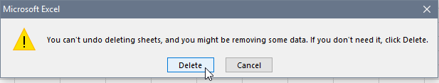
Delete Sheet Warning

Between Sheet Deleted
Copy Sheet
A sheet can be copied by using the command sheets("SHEETNAME").Copy. The code below copies the sheet to the location after the last sheet using the After:=sheets(sheets.Count) command. Note the (2) after in the sheet name signifying it is a copy.
Input:sheets("BETWEENTESTSHEET").Copy After:=sheets(sheets.Count)

Copy Sheet
Output:
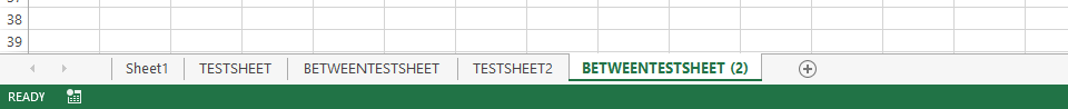
Copy Sheet Copied
Rename Sheet
A sheet can be renamed by using the command sheets("CURRENTNAME").Name = "NEWNAME".
Input:sheets("BETWEENTESTSHEET (2)").Name = "RENAMEDSHEET"
Copy Sheet Renaming
Output:
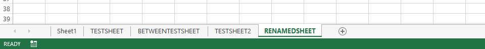
Sheet Renamed
Sheet Cells
Now that there are multiple sheets in this Excel Workbook, one must specify a sheet in order to modify that specific sheet's cells. Modifying cells without a sheet callout only modifies cells for the current active sheet; this is the sheet that is currently selected.
Input:Cells(1, 1) = 1
Output:
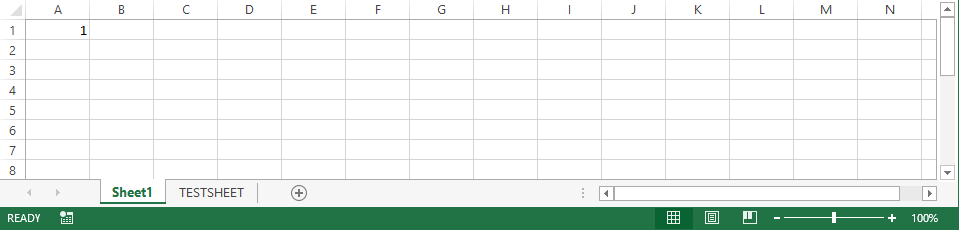
Selected Sheet
Not Selected Sheet
One would have to state what sheet is to be modified with the sheets("SHEETNAME").Cells(ROW, COLUMN) command. This method allows for the modification of cells in sheets even if the specified sheets are not selected.
Input:sheets("Sheet1").Cells(1, 1) = 1
sheets("TESTSHEET").Cells(1, 1) = 1
Output:
Selected Sheet
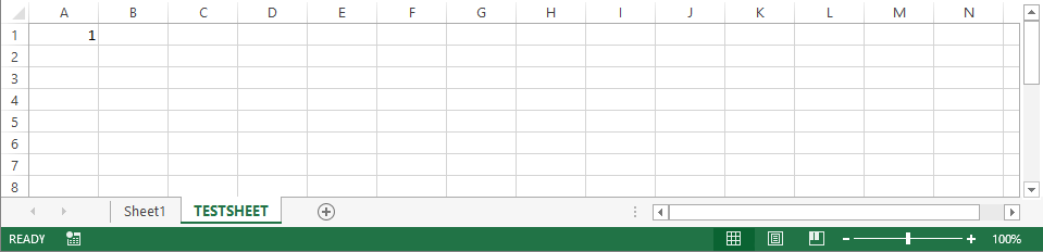
Not Selected Sheet Modified
The sheet name must also be declared when clearing the cells.
Input:sheets("Sheet1").Cells.ClearContents
sheets("Sheet1").Cells.ClearFormats
sheets("Sheet1").Cells.RowHeight = 15
sheets("Sheet1").Cells.ColumnWidth = 8.43
sheets("TESTSHEET").Cells.ClearContents
sheets("TESTSHEET").Cells.ClearFormats
sheets("TESTSHEET").Cells.RowHeight = 15
sheets("TESTSHEET").Cells.ColumnWidth = 8.43
However, the Range command is a bit different as the sheet must be specified for the cells and not the range.
Input:Range(sheets("Sheet1").Cells(1, 1), sheets("Sheet1").Cells(5, 5)) = 1
Range(sheets("TESTSHEET").Cells(1, 1), sheets("TESTSHEET").Cells(5, 5)) = 1
Output:
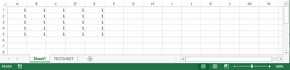
Selected Sheet
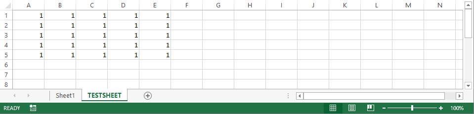
Not Selected Sheet Modified
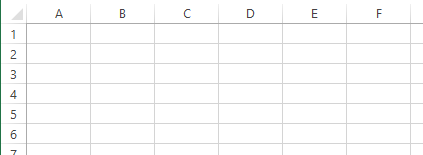
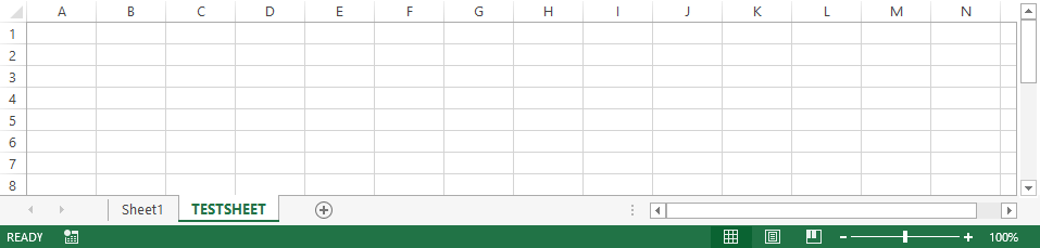
An error will occur if the sheets("SHEETNAME").Range command is used and the sheet SHEETNAME is not the one currently active.
Input:sheets("Sheet1").Range(Cells(1, 1), Cells(5, 5)) = 1
sheets("TESTSHEET").Range(Cells(1, 1), Cells(5, 5)) = 1
Output:
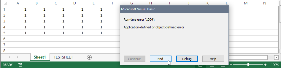
Range Error
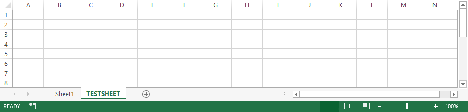
Empty Sheet
You can now modify and customize cells using the commands in the Cells section.
Input:Range(sheets("Sheet1").Cells(1, 1), sheets("Sheet1").Cells(5, 5)) = 1
Range(sheets("TESTSHEET").Cells(1, 1), sheets("TESTSHEET").Cells(5, 5)) = 1
Range(sheets("Sheet1").Cells(1, 1), sheets("Sheet1").Cells(5, 5)).Interior.Color = RGB(125, 0, 0)
Range(sheets("TESTSHEET").Cells(1, 1), sheets("TESTSHEET").Cells(5, 5)).Interior.Color = RGB(125, 0, 0)
Output:
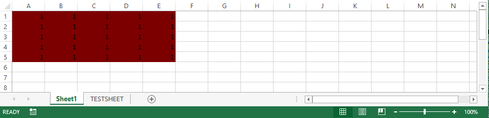
Sheet1 Color
TESTSHEET Color
Copy Cells from Sheets
Copying cells from one sheet is done by using the .Copy command and pasting them into another sheet is done by using the .PasteSpecial command. Note that only the top left cell (in this case Cells(1,1)) needs to be stated for the pasting location.
Input:Range(sheets("Sheet1").Cells(1, 1), sheets("Sheet1").Cells(5, 5)) = 5
Range(sheets("Sheet1").Cells(1, 1), sheets("Sheet1").Cells(5, 5)).Interior.Color = RGB(125, 0, 0)
Range(sheets("Sheet1").Cells(1, 1), sheets("Sheet1").Cells(5, 5)).Copy
sheets("TESTSHEET").Cells(1, 1).PasteSpecial
Output:

Copy Range
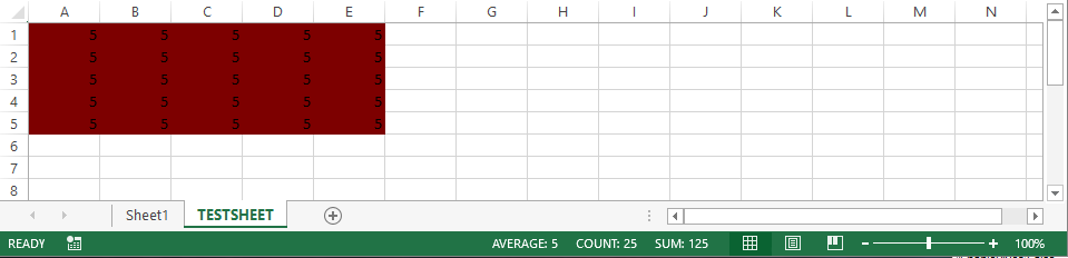
Paste Range
Charts
Excel VBA can be used to create charts in order to make the process of presenting data a lot faster. One can automatically select the data, name the chart, select the chart type, etc. using VBA instead of manually going through the Insert tab.
Creating Charts
The first step in creating a chart is to add a chart using the .Shapes.AddChart command. The .Select command will select the chart in order to use the With command in a bit.
Input:sheets("Sheet1").Shapes.AddChart.Select
Output:
Blank Chart
All charts can be deleted with the command below. This command will give an error if there are no charts on the specified sheet.
Input:sheets("Sheet1").ChartObjects.Delete
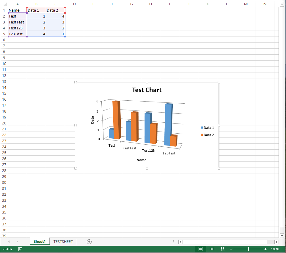
Now we will select the data and give this chart a title. It is important to note that if no data is selected, the chart will remain blank without a title. The default chart type in excel is a column chart if one does not specify a chart type. The data series will be named according to the header column if the header column is included in the range.
Input:sheets("Sheet1").Shapes.AddChart.Select
With ActiveChart
.SetSourceData Source:=Range(sheets("Sheet1").Cells(1, 1), sheets("Sheet1").Cells(5, 3))
.HasTitle = True
.ChartTitle.Text = "Test Chart"
End With
Output:
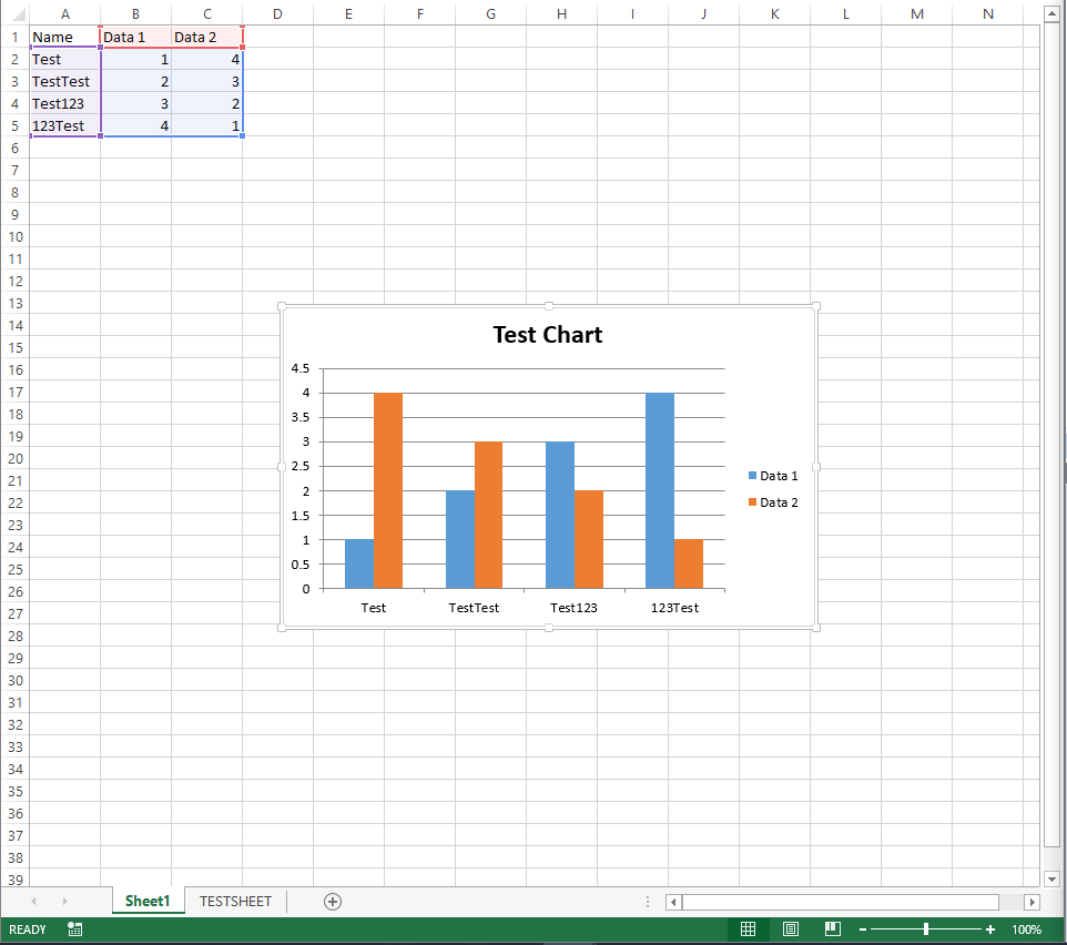
New Chart
The chart type can be selected using the .ChartType command. For a list of all the other chart types, please see this Microsoft Chart Type Page.
Input:sheets("Sheet1").Shapes.AddChart.Select
With ActiveChart
.SetSourceData Source:=Range(sheets("Sheet1").Cells(1, 1), sheets("Sheet1").Cells(5, 3))
.HasTitle = True
.ChartTitle.Text = "Test Chart"
.ChartType = xl3DColumnClustered
End With
Output:
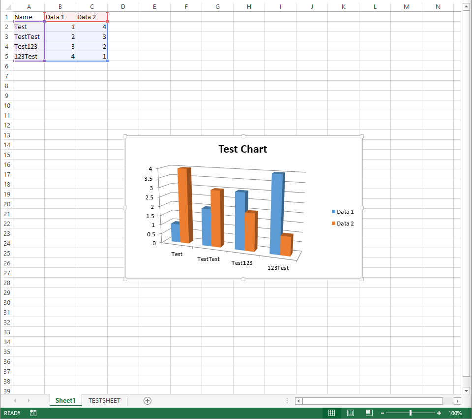
New Chart
The axes can be given names with the .Axes command. The xlCategory is the X-Axis while the xlValue is the Y-Axis.
Input:sheets("Sheet1").Shapes.AddChart.Select
With ActiveChart
.SetSourceData Source:=Range(sheets("Sheet1").Cells(1, 1), sheets("Sheet1").Cells(5, 3))
.HasTitle = True
.ChartTitle.Text = "Test Chart"
.ChartType = xl3DColumnClustered
.Axes(xlCategory, xlPrimary).HasTitle = True
.Axes(xlCategory, xlPrimary).AxisTitle.Text = "Name"
.Axes(xlValue, xlPrimary).HasTitle = True
.Axes(xlValue, xlPrimary).AxisTitle.Text = "Data"
End With
Output:
Axes Titles
The series can be modified with the .SeriesCollection() commands below. The number in the .SeriesCollection() corresponds to the order of the plotted data. I have renamed the data series with .Name and changed the color with .Interior.Color.
Input:sheets("Sheet1").Shapes.AddChart.Select
With ActiveChart
.SetSourceData Source:=Range(sheets("Sheet1").Cells(1, 1), sheets("Sheet1").Cells(5, 3))
.HasTitle = True
.ChartTitle.Text = "Test Chart"
.ChartType = xl3DColumnClustered
.Axes(xlCategory, xlPrimary).HasTitle = True
.Axes(xlCategory, xlPrimary).AxisTitle.Text = "Name"
.Axes(xlValue, xlPrimary).HasTitle = True
.Axes(xlValue, xlPrimary).AxisTitle.Text = "Data"
.SeriesCollection(1).Name = "Data One"
.SeriesCollection(1).Interior.Color = RGB(250, 0, 0)
.SeriesCollection(2).Name = "Data Two"
.SeriesCollection(2).Interior.Color = RGB(0, 250, 0)
End With
Output:
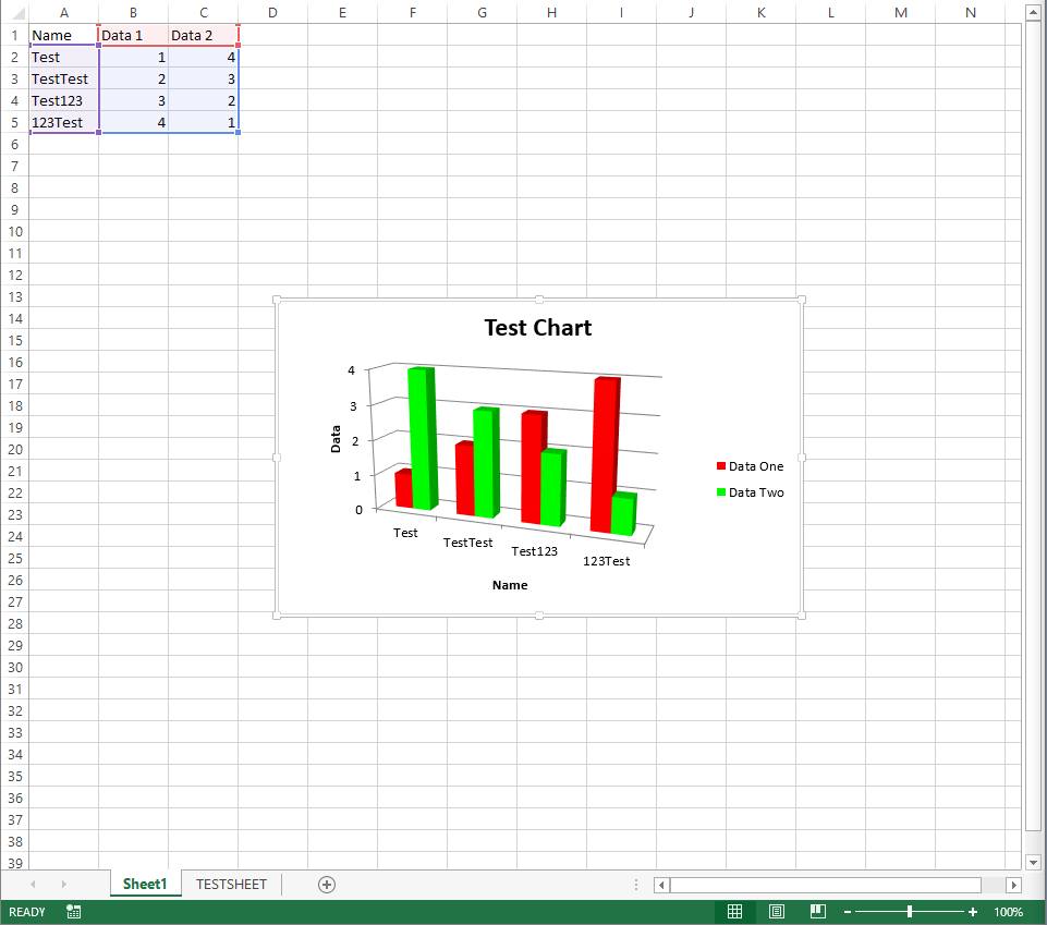
Modifying Series
The chart location and size can be modified with the .Parent command. The .Top range only depends on the row and states the top position location of the chart. The .Left range only depends on the column and states the left position location of the chart. I have selected the top position of the chart to be located on row 10 and the left position of the chart to be located on column E. The .Height and .Width adjust the height and width of the chart, respectively. The height of the chart spans from row 10 to row 30 (E10 to E30) while the width of the chart spans from column E to column N (E10 to N10).
Input:sheets("Sheet1").Shapes.AddChart.Select
With ActiveChart
.SetSourceData Source:=Range(sheets("Sheet1").Cells(1, 1), sheets("Sheet1").Cells(5, 3))
.HasTitle = True
.ChartTitle.Text = "Test Chart"
.ChartType = xl3DColumnClustered
.Axes(xlCategory, xlPrimary).HasTitle = True
.Axes(xlCategory, xlPrimary).AxisTitle.Text = "Name"
.Axes(xlValue, xlPrimary).HasTitle = True
.Axes(xlValue, xlPrimary).AxisTitle.Text = "Data"
.SeriesCollection(1).Name = "Data One"
.SeriesCollection(1).Interior.Color = RGB(250, 0, 0)
.SeriesCollection(2).Name = "Data Two"
.SeriesCollection(2).Interior.Color = RGB(0, 250, 0)
.Parent.Top = Range("A10").Top
.Parent.Left = Range("E1").Left
.Parent.Height = Range("E10:E30").Height
.Parent.Width = Range("E10:N10").Width
End With
Output:
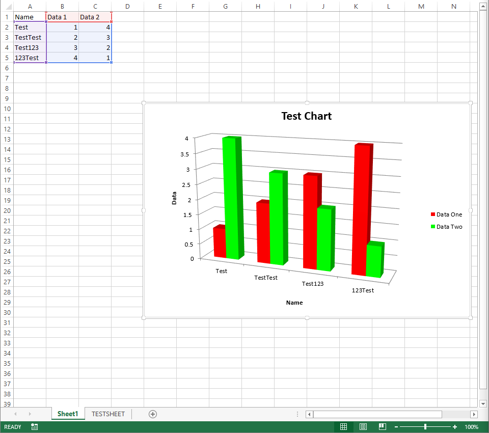
Chart Location and Size
Additional data can be added to a chart even if the data is not next to the other data. The Union command combines different ranges in order for all the data to be included in the chart. In the image below, I have created another range which covers the third data set (Range(sheets("Sheet1").Cells(1, 5), sheets("Sheet1").Cells(5, 5))) and appended it to the other ranges with the Union command by separating it from the first range with a comma.
Input:sheets("Sheet1").Shapes.AddChart.Select
With ActiveChart
.SetSourceData Source:=Union(Range(sheets("Sheet1").Cells(1, 1), sheets("Sheet1").Cells(5, 3)), Range(sheets("Sheet1").Cells(1, 5), sheets("Sheet1").Cells(5, 5)))
.HasTitle = True
.ChartTitle.Text = "Test Chart"
.ChartType = xl3DColumnClustered
.Axes(xlCategory, xlPrimary).HasTitle = True
.Axes(xlCategory, xlPrimary).AxisTitle.Text = "Name"
.Axes(xlValue, xlPrimary).HasTitle = True
.Axes(xlValue, xlPrimary).AxisTitle.Text = "Data"
.SeriesCollection(1).Name = "Data One"
.SeriesCollection(1).Interior.Color = RGB(250, 0, 0)
.SeriesCollection(2).Name = "Data Two"
.SeriesCollection(2).Interior.Color = RGB(0, 250, 0)
.SeriesCollection(3).Name = "Data Three"
.SeriesCollection(3).Interior.Color = RGB(0, 0, 250)
.Parent.Top = Range("A10").Top
.Parent.Left = Range("E1").Left
.Parent.Height = Range("E10:E30").Height
.Parent.Width = Range("E10:N10").Width
End With
Output:
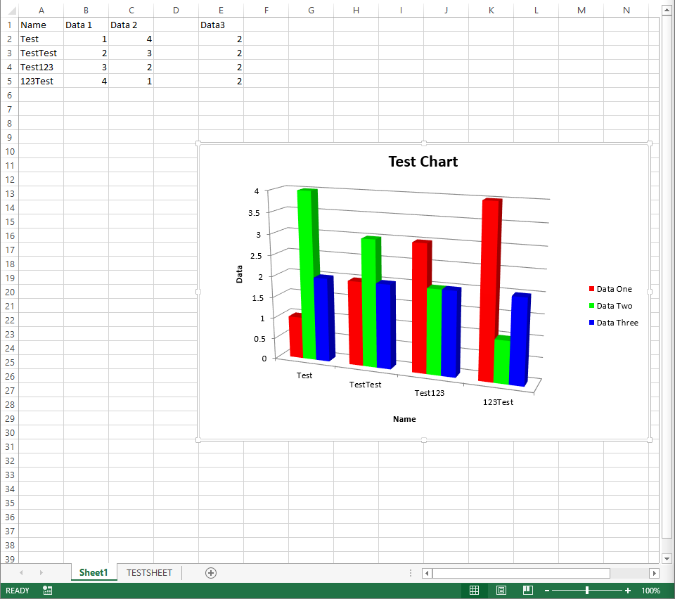
Additional Range
Scatter Plot with Lines
Creating a scatter plot with lines (.ChartType = xlXYScatterLines) is a bit different than creating a column graph. Each series is individually created by using .SeriesCollection.NewSeries. The X Values are assigned using .SeriesCollection(#).XValues and the Y Values are assigned using .SeriesCollection(#).Values. The line color, line weight, and dash style are modified using .Format.Line.ForeColor.RGB, .Format.Line.Weight, and .Format.Line.DashStyle (Dash Styles), respectively. The marker color, size, and style are modified using .MarkerBackgroundColor, .MarkerSize, and .MarkerStyle (Marker Styles), respectively. For a much more efficient way of creating each of these new series, please see the Loop Chart section.
Input:sheets("Sheet1").Shapes.AddChart.Select
With ActiveChart
.HasTitle = True
.ChartTitle.Text = "Test Chart"
.ChartType = xlXYScatterLines
.Axes(xlCategory, xlPrimary).HasTitle = True
.Axes(xlCategory, xlPrimary).AxisTitle.Text = "X Values"
.Axes(xlValue, xlPrimary).HasTitle = True
.Axes(xlValue, xlPrimary).AxisTitle.Text = "Data"
.SeriesCollection.NewSeries
.SeriesCollection(1).Name = "Data One"
.SeriesCollection(1).XValues = Range(sheets("Sheet1").Cells(2, 1), sheets("Sheet1").Cells(5, 1))
.SeriesCollection(1).Values = Range(sheets("Sheet1").Cells(2, 2), sheets("Sheet1").Cells(5, 2))
.SeriesCollection(1).Format.Line.ForeColor.RGB = RGB(250, 0, 0)
.SeriesCollection(1).Format.Line.Weight = 5
.SeriesCollection(1).MarkerBackgroundColor = RGB(125, 0, 0)
.SeriesCollection(1).MarkerSize = 50
.SeriesCollection(1).MarkerStyle = xlMarkerStyleCircle
.SeriesCollection.NewSeries
.SeriesCollection(2).Name = "Data Two"
.SeriesCollection(2).XValues = Range(sheets("Sheet1").Cells(2, 1), sheets("Sheet1").Cells(5, 1))
.SeriesCollection(2).Values = Range(sheets("Sheet1").Cells(2, 3), sheets("Sheet1").Cells(5, 3))
.SeriesCollection(2).Format.Line.ForeColor.RGB = RGB(0, 250, 0)
.SeriesCollection(2).Format.Line.Weight = 2
.SeriesCollection(2).Format.Line.DashStyle = msoLineDash
.SeriesCollection(2).MarkerBackgroundColor = RGB(0, 125, 0)
.SeriesCollection(2).MarkerSize = 70
.SeriesCollection(2).MarkerStyle = xlMarkerStyleDiamond
.SeriesCollection.NewSeries
.SeriesCollection(3).Name = "Data Three"
.SeriesCollection(3).XValues = Range(sheets("Sheet1").Cells(2, 1), sheets("Sheet1").Cells(5, 1))
.SeriesCollection(3).Values = Range(sheets("Sheet1").Cells(2, 5), sheets("Sheet1").Cells(5, 5))
.SeriesCollection(3).Format.Line.ForeColor.RGB = RGB(0, 0, 250)
.SeriesCollection(3).Format.Line.Weight = 2
.SeriesCollection(3).Format.Line.DashStyle = msoLineDashDot
.SeriesCollection(3).MarkerBackgroundColor = RGB(0, 0, 125)
.SeriesCollection(3).MarkerSize = 25
.SeriesCollection(3).MarkerStyle = xlMarkerStyleSquare
.Parent.Top = Range("A10").Top
.Parent.Left = Range("E1").Left
.Parent.Height = Range("E10:E30").Height
.Parent.Width = Range("E10:N10").Width
End With
Output:
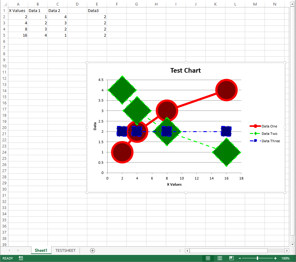
Scatter Plot with Lines
Pie Chart
A pie chart can be created using .ChartType = xlPie. The range of the data includes the headers in order for the series to be labeled accordingly. Data labels are created using the .ApplyDataLabels command. The position, shape, and visibility of the data labels are modified with .SeriesCollection(#).DataLabels.Position (Data Label Positions), .SeriesCollection(#).DataLabels.Format.AutoShapeType (Data Label Shapes), and .SeriesCollection(#).DataLabels.Format.Line.Visible, respectively. The color of each data point is changed using .SeriesCollection(#).Points(#).Format.Fill.ForeColor.RGB. Note that the series collection number is (1) for all of the points while the points' number changes.
Input:sheets("Sheet1").Shapes.AddChart.Select
With ActiveChart
.SetSourceData Source:=Range(sheets("Sheet1").Cells(1, 1), sheets("Sheet1").Cells(5, 2))
.HasTitle = True
.ChartTitle.Text = "Test Chart"
.ChartType = xlPie
.ApplyDataLabels (xlDataLabelsShowLabelAndPercent)
.SeriesCollection(1).DataLabels.Position = xlLabelPositionOutsideEnd
.SeriesCollection(1).DataLabels.Format.AutoShapeType = msoShapeRectangularCallout
.SeriesCollection(1).DataLabels.Format.Line.Visible = msoTrue
.SeriesCollection(1).Points(1).Format.Fill.ForeColor.RGB = RGB(250, 0, 0)
.SeriesCollection(1).Points(2).Format.Fill.ForeColor.RGB = RGB(0, 250, 0)
.SeriesCollection(1).Points(3).Format.Fill.ForeColor.RGB = RGB(0, 0, 250)
.SeriesCollection(1).Points(4).Format.Fill.ForeColor.RGB = RGB(125, 125, 125)
.Parent.Top = Range("A10").Top
.Parent.Left = Range("E1").Left
.Parent.Height = Range("E10:E30").Height
.Parent.Width = Range("E10:N10").Width
End With
Output:
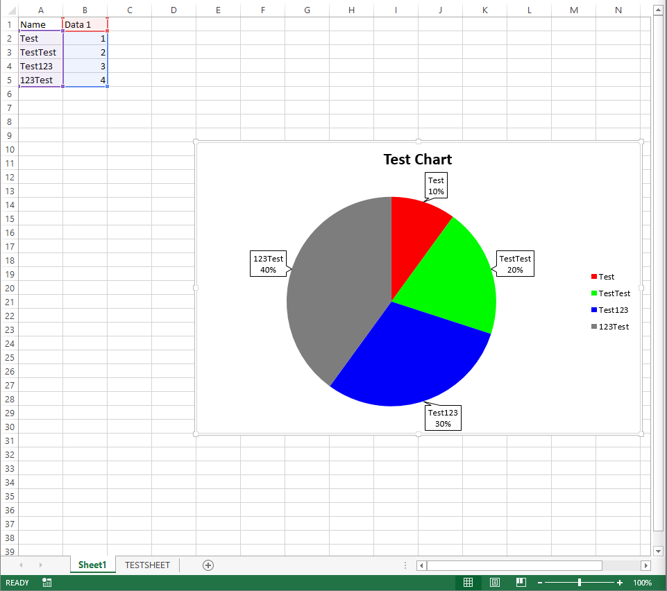
Pie Chart
Useful Commands
This section will cover some of the commands that I have found useful over the years.
- For Loop
- If Statement
- Sum and Average
- User Input
- Last Row and Last Column
- Loop Chart
- Match
- Hide
- Auto Filter
- Screen Updating
- Master Subroutine
- Macro Button
For Loop
A for loop is very useful if one has to iterate through a lot of cells. The loop below uses the counter i to count from 1 to 10. The code assigns "Row" to rows 2 through 11 in column 1 by having the counter i+1 in the row position while keeping column 1 static. The code also assigns "Column" to columns 2 through 11 in row 1 by having the counter i+1 in the column position while keeping row 1 static.
Input:For i = 1 To 10
sheets("Sheet1").Cells(i + 1, 1) = "Row"
sheets("Sheet1").Cells(1, i + 1) = "Column"
Next i
Output:
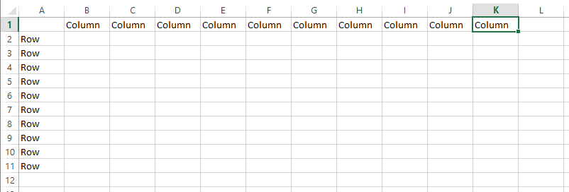
For Loop
A for loop can be within another for loop as seen below. These loops have two counters (i and j) which allows them to iterate through both rows and columns. The outer loop counter is static until the inner loop finishes. After the inner loop finishes, the outer loop counter increases and the inner loop counts again. This loop starts out at i = 1 and loops through j = 1 to 10. Afterwards, the i counter increases to i = 2 and loops through j = 1 to 10 again and so on. In the example below, row 1 columns 1 through 10 are assigned a value of 1. Then, row 2 columns 1 through 10 are assigned a value of 1 and so on.
Input:For i = 1 To 10
For j = 1 To 10
sheets("Sheet1").Cells(i, j) = 1
Next j
Next i
Output:
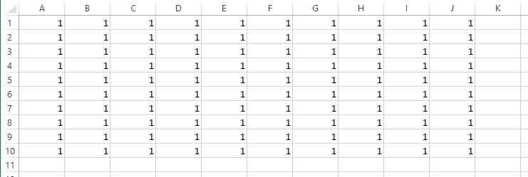
Embedded For Loop
If Statement
The if statement is very useful if you want to check for certain criteria in cells. Below is an if statement inside a for loop that checks rows 1 through 10 in column 1 for certain criteria. The first if statement changes the cell color of the cell to red if the value is less than 10. The elseif statement changes the cell color of the cell to green if the value is greater than or equal to 10. The first if statement that a cell meets will be applied to that cell. As seen below, a third statement repeats the first statement but with a different color change. However, the modification does not get applied as the cells have already met a criteria beforehand.
Input:For i = 1 To 10
If sheets("Sheet1").Cells(i, 1) < 10 Then
sheets("Sheet1").Cells(i, 1).Interior.Color = RGB(250, 0, 0)
ElseIf sheets("Sheet1").Cells(i, 1) >= 10 Then
sheets("Sheet1").Cells(i, 1).Interior.Color = RGB(0, 250, 0)
ElseIf sheets("Sheet1").Cells(i, 1) < 10 Then
sheets("Sheet1").Cells(i, 1).Interior.Color = RGB(0, 0, 250)
End If
Next i
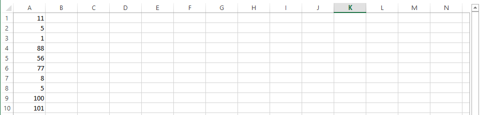
Simple If Statement Not Executed
Output:
Simple If Statement Executed
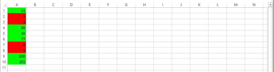
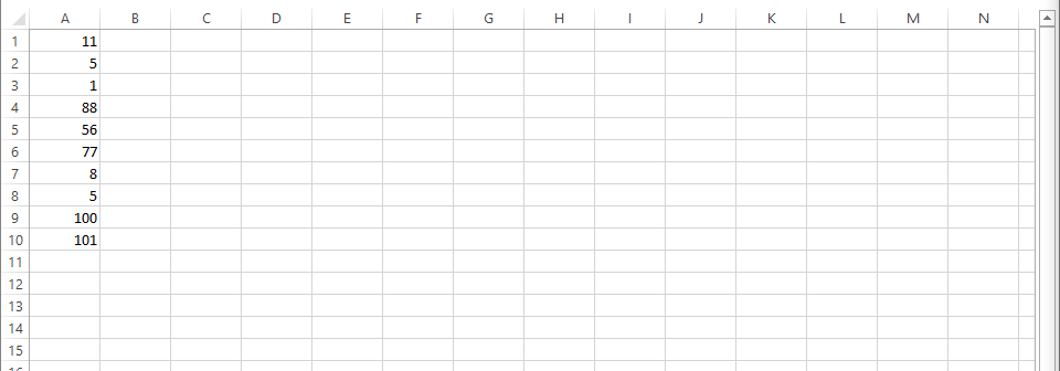
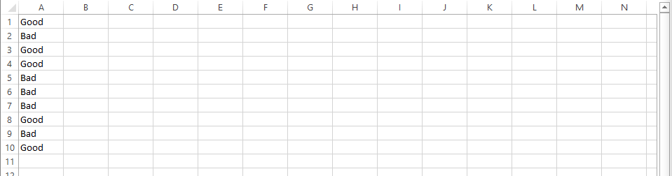
Below is more complicated if statement inside a for loop that checks rows 1 through 15 in column 1 for certain criteria and then modifies the cells accordingly.
The first if statement checks if the cell is less than 10 AND is not empty (empty gives true for a value of 0) and changes the cell color to red.
The first elseif statement checks if the cell value is greater than or equal to 10 AND if it is less than 100 and changes the cell color to green.
The second elseif statement checks if the value is equal to 100 and changes the cell color to blue.
The third elseif statement checks if the value is greater than or equal to 100 and if it is numeric (string also gives a value greater than 100) and changes the cell color to gray.
The else statement gives everything else a value of "Blank." In this case, rows 11-15 do not fit any of the criteria in the other if statements above.
An example OR statement would be: If sheets("Sheet1").Cells(i, 1) < 10 Or Not IsEmpty(sheets("Sheet1").Cells(i, 1)) Then.
For i = 1 To 15

								 If sheets("Sheet1").Cells(i, 1) < 10 And Not IsEmpty(sheets("Sheet1").Cells(i, 1)) Then

									sheets("Sheet1").Cells(i, 1).Interior.Color = RGB(250, 0, 0)


									ElseIf sheets("Sheet1").Cells(i, 1) >= 10 And sheets("Sheet1").Cells(i, 1) < 100 Then

									sheets("Sheet1").Cells(i, 1).Interior.Color = RGB(0, 250, 0)


									ElseIf sheets("Sheet1").Cells(i, 1) = 100 Then

									sheets("Sheet1").Cells(i, 1).Interior.Color = RGB(0, 0, 250)


									ElseIf sheets("Sheet1").Cells(i, 1) >= 100 And IsNumeric(sheets("Sheet1").Cells(i, 1)) Then

									sheets("Sheet1").Cells(i, 1).Interior.Color = RGB(125, 125, 125)


									Else

									sheets("Sheet1").Cells(i, 1) = "Blank"


								End If
							Next i
If Statement Not Executed
Output:
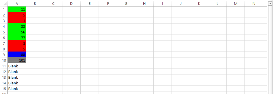
If Statement Executed
Sum and Average
The code for the sum and average of a range can be seen below. I have also made certain cells have the string Sum: and Average: in order for the values to have a label.
Input:sheets("Sheet1").Cells(15, 1) = "Sum:"
sheets("Sheet1").Cells(16, 1) = "Average:"
sheets("Sheet1").Cells(15, 2) = Application.WorksheetFunction.Sum(Range(sheets("Sheet1").Cells(1, 1), sheets("Sheet1").Cells(10, 1)))
sheets("Sheet1").Cells(16, 2) = Application.WorksheetFunction.Average(Range(sheets("Sheet1").Cells(1, 1), sheets("Sheet1").Cells(10, 1)))
Output:
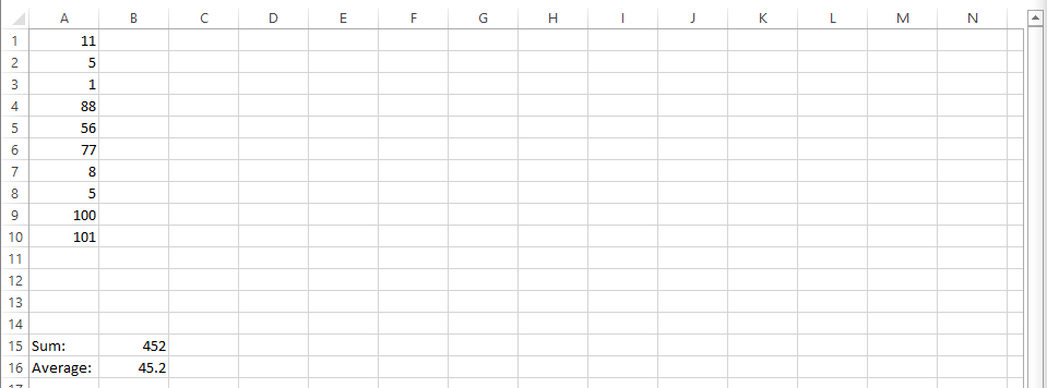
Sum and Average
User Input
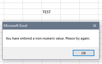
Excel VBA can also ask for user input. The code below asks for the user's input using InputBox("Message", "Message Title") and assigns it to a certain cell. The code then uses a While loop to keep checking if the input is numeric. A while loop does not end until the criteria is met. Inside the while loop, a Message Box (MsgBox) pops up telling the user that the input was not numeric and then the code asks for the user's input again. The while loop keeps repeating until the user inputs a numeric value.
Input:UserInput = InputBox("Enter a Value", "Input Message Title Goes Here")
sheets("Sheet1").Cells(10, 10) = UserInput
While Not IsNumeric(sheets("Sheet1").Cells(10, 10))
MsgBox "You have entered a non-numeric value. Please try again."
UserInput = InputBox("Enter a Value", "Input Message Title Goes Here")
sheets("Sheet1").Cells(10, 10) = UserInput
Wend
Output:
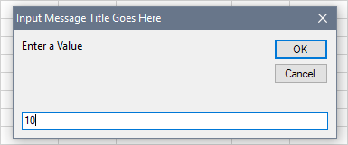
Input Message
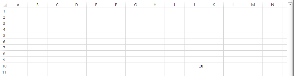
Input Message Success
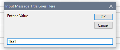
Input Message String
Input Message Error
Last Row and Last Column
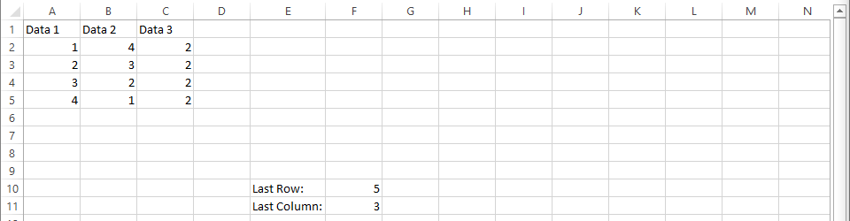
Acquiring the last row and last column of a data set is tremendously useful as one can create variables using those values which allows the Excel VBA code to adjust according to the data size. The Rows.Count and Columns.Count commands give the total number of rows and columns in a sheet, respectively. The .End(xlDIRECTION) moves the cell selection in the specified direction until it sees a non-empty cell. The .Row and .Column commands return the row and column of that specified cell, respectively. In the code below, the lastrow variable is moving up from the very last row in column 1 until it finds the first non-empty row which is the last row of the dataset. The same is happening with the lastcolumn variable except it uses columns instead of rows.
Input:lastrow = sheets("Sheet1").Cells(Rows.Count, 1).End(xlUp).Row
lastcolumn = sheets("Sheet1").Cells(1, Columns.Count).End(xlToLeft).Column
sheets("Sheet1").Cells(10, 5) = "Last Row:"
sheets("Sheet1").Cells(10, 6) = lastrow
sheets("Sheet1").Cells(11, 5) = "Last Column:"
sheets("Sheet1").Cells(11, 6) = lastcolumn
Output:
Last Row and Column
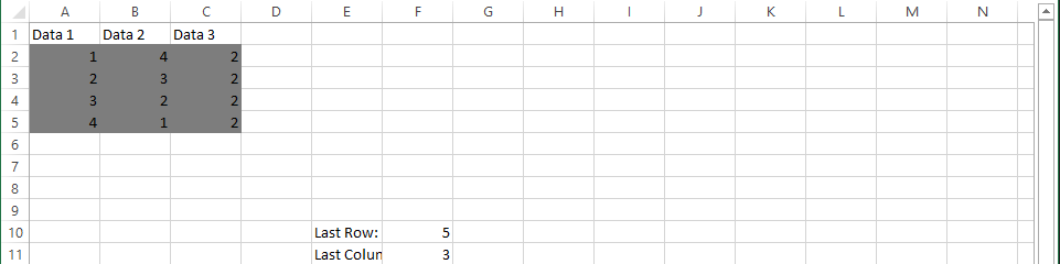
Dynamic counters for the for loops can now be created using the lastrow and lastcolumn variables. This makes it a lot easier to go through all the data in a table even if the data table changes size. In the code below, the rows start at i = 2 since row 1 is the header row and continues to lastrow. The columns start at j = 1 and continues to lastcolumn.
Input:For i = 2 To lastrow
For j = 1 To lastcolumn
sheets("Sheet1").Cells(i, j).Interior.Color = RGB(125, 125, 125)
Next j
Next i
Output:
Last Row and Column Loop
Loop Chart
Another very useful VBA code that combines for loops with the lastrow and lastcolumn variables is a code that creates charts. As seen in the Scatter Plot with Lines section, using .SeriesCollection.NewSeries for every new series can make the code really large. Using for loops with the lastrow and lastcolumn variables reduces the size of the code significantly especially if you have +10 series.
In the code below, there is a for loop for the creation of each new series. The loop starts at column 2 since the first column contains the X values and continues to lastcolumn. The .SeriesCollection(#) number is i-1 since i starts at 2. The X values are in column one and the rows of the values range from row 2 to lastrow since the first row is the header. The values of each series are in column i and the rows range from row 2 to lastrow since the first row contains the headers. This makes the chart creation a lot shorter and less tedious by not having to input each new series individually.
Input:sheets("Sheet1").Shapes.AddChart.Select
With ActiveChart
.HasTitle = True
.ChartTitle.Text = "Test Chart"
.ChartType = xlXYScatterLines
.Axes(xlCategory, xlPrimary).HasTitle = True
.Axes(xlCategory, xlPrimary).AxisTitle.Text = "X Values"
.Axes(xlValue, xlPrimary).HasTitle = True
.Axes(xlValue, xlPrimary).AxisTitle.Text = "Data"
For i = 2 To lastcolumn
.SeriesCollection.NewSeries
.SeriesCollection(i - 1).Name = sheets("Sheet1").Cells(1, i)
.SeriesCollection(i - 1).XValues = Range(sheets("Sheet1").Cells(2, 1), sheets("Sheet1").Cells(lastrow, 1))
.SeriesCollection(i - 1).Values = Range(sheets("Sheet1").Cells(2, i), sheets("Sheet1").Cells(lastrow, i))
Next i
End With
Output:
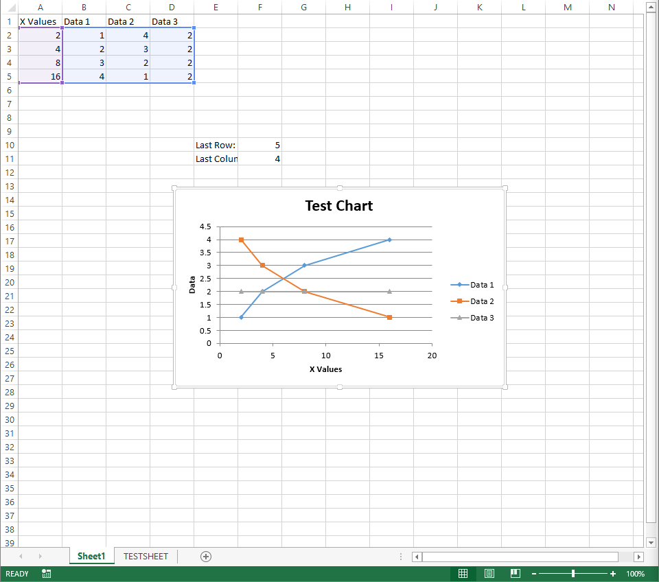
Last Row and Column Chart
Match
One can find specific columns of data using the .Match command. Once you have found a specific data column, you can use that column number as a variable to modify those cells. The code below looks for an exact match (0) of the string "Data #" in the specified range of the first row from the first column up to last column. The code then uses that column number to modify the color of each of those cells.
Input:Data1Column = Application.WorksheetFunction.Match("Data 1", Range(sheets("Sheet1").Cells(1, 1), sheets("Sheet1").Cells(1, lastcolumn)), 0)
Data2Column = Application.WorksheetFunction.Match("Data 2", Range(sheets("Sheet1").Cells(1, 1), sheets("Sheet1").Cells(1, lastcolumn)), 0)
Data3Column = Application.WorksheetFunction.Match("Data 3", Range(sheets("Sheet1").Cells(1, 1), sheets("Sheet1").Cells(1, lastcolumn)), 0)
sheets("Sheet1").Cells(1, Data1Column).Interior.Color = RGB(250, 0, 0)
sheets("Sheet1").Cells(1, Data2Column).Interior.Color = RGB(0, 250, 0)
sheets("Sheet1").Cells(1, Data3Column).Interior.Color = RGB(0, 0, 250)
Output:
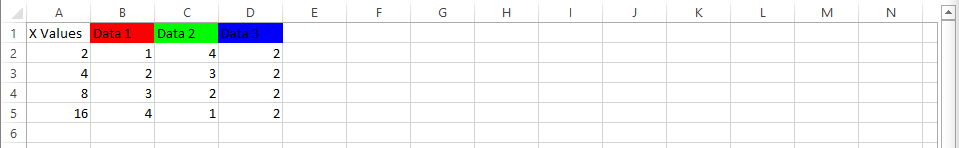
Last Row and Column Match
Hide
Rows and columns can be hidden with the .Hidden command. The code below loops through rows 1 through 10 in column 1 and hides any cells' rows that meet a certain criteria.
Input:For i = 1 To lastrow
If sheets("Sheet1").Cells(i, 1) = "Bad" Then
sheets("Sheet1").Rows(i).EntireRow.Hidden = True
End If
Next i
Hiding Rows
Output:
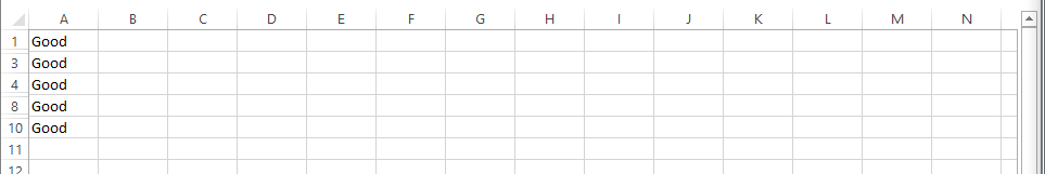
Hidden Rows
You can unhide the rows by making the statement "False" in the .Hidden command.
Input:sheets("Sheet1").Rows.EntireRow.Hidden = False
The code below loops through columns 1 through 10 in row 1 and hides any cells' columns that meet a certain criteria.
Input:For i = 1 To lastcolumn
If sheets("Sheet1").Cells(1, i) = "Bad" Then
sheets("Sheet1").Columns(i).EntireColumn.Hidden = True
End If
Next i

Hiding Columns
Output:

Hidden Columns
You can unhide the columns by making the statement "False" in the .Hidden command.
Input:sheets("Sheet1").Columns.EntireColumn.Hidden = False
Auto Filter
Filters can be added to the header row by using the .AutoFilter command.
Input:Range(sheets("Sheet1").Cells(1, 1), sheets("Sheet1").Cells(1, lastcolumn)).AutoFilter
Output:
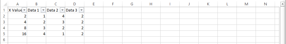
Filter
Screen Updating
If you have a large Excel VBA code, updating your screen every time a command executes can slow down your macro. Using the Application.ScreenUpdating = False can help execute your code in less time. Place your code in between Application.ScreenUpdating = False and Application.ScreenUpdating = True.
Input:Sub TESTSUB()
Application.ScreenUpdating = False
*** THE REST OF YOUR CODE GOES HERE ***
Application.ScreenUpdating = True
End Sub
Master Subroutine
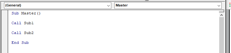
Creating multiple subroutines is useful if one would want to declutter their macros. Subroutines can be executed within another subroutine by using the Call command. Here, the Master subroutine calls two other subroutines: Sub1 and Sub2. These subroutines can be within the same module or different modules.
Input:Sub Master()
Call Sub1
Call Sub2
End Sub

Master Sub Same Module
Master Sub Different Module
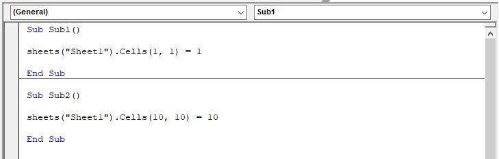
Subs Different Module
Output:
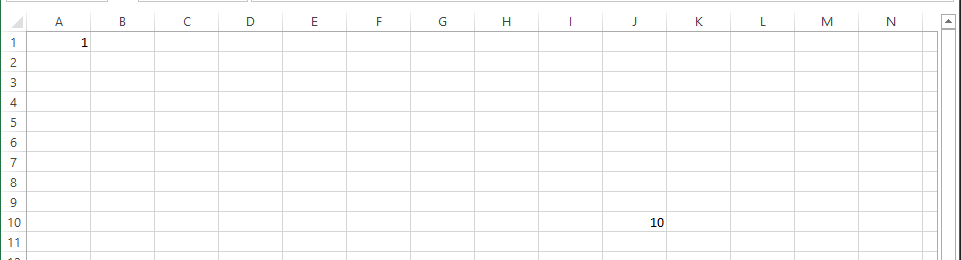
Sub Call
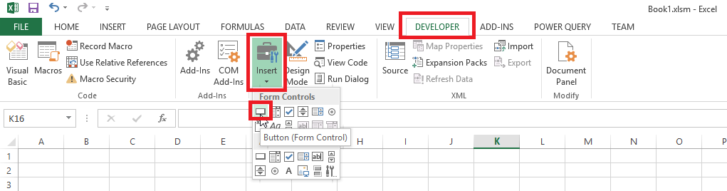
Macro Button
Adding macro buttons to a sheet for quick access to a macro can be done by going to the Developer tab, selecting Insert, and clicking on Button. The button size will then be adjustable by dragging the mouse to the desired size. Right clicking on the button will allow the user to edit it. Left clicking on the sheet and then on the button will run the macro.
Create Button
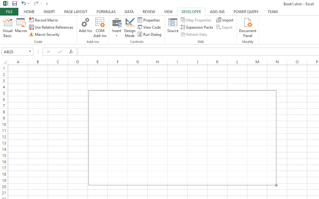
Create Button Size
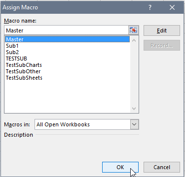
Assign Macro
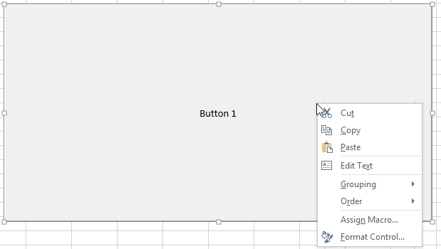
Right Click to Edit Button
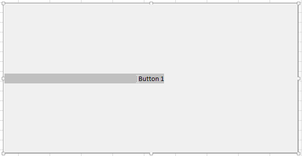
Rename Button
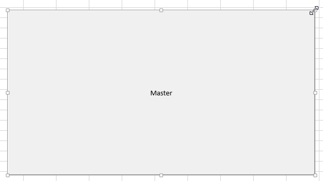
Resize Button
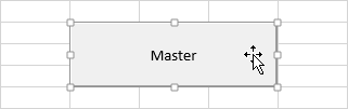
Move Button
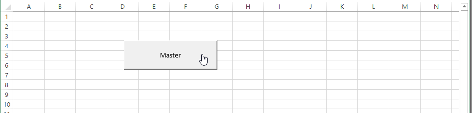
Click Button
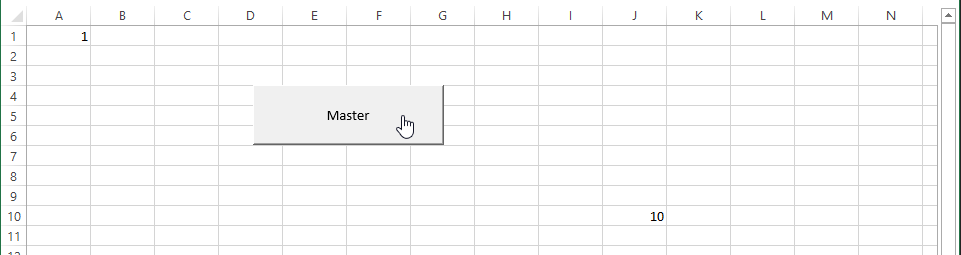
Button Clicked