Linear Regression with Gradient Descent
Introduction
This tutorial will use Python to apply a linear fit on some data using linear regression and gradient descent. Gradient descent is an algorithm that finds the minimum of a function, in this case, the cost function of the linear regression model. Minimizing the cost function will produce a linear fit with the least error which allows better prediction of y given x. The Python code can be downloaded from my GitHub page. The data set can be downloaded from Kaggle.
Gradient Descent
The method that will be used to find the minimum of the cost function is the gradient descent algorithm. This algorithm works by first picking a point, finding the slope of the function at that point, and then moving the point towards the minimum now knowing the slope of the function at that point. For example, if the current point has a positive slope, the next iteration will have the point to the left of the initial point since a minimum will most likely be found moving against the positive slope. If the current point has a negative slope, the next iteration will have the point to the right of the initial point since a minimum will most likely be found moving with the negative slope. This process is repeated until the minimum of the function is found. The generic equation for the gradient descent algorithm can be seen below.
$$x_{n+1}= x_n - \alpha \nabla F(x_n)$$
Where $x_{n}$ is the current point, $ \alpha $ is the step size, $ \nabla F(x_n)$ is the gradient of the function at $x_{n}$, and $x_{n+1}$ is the next point of the iteration. Note that choosing a small enough step size is important so that the minimum does not get overshot (but not too small as the iterative process will take a long time). An example of the gradient descent algorithm being applied to the function $y=x^2 $ can be seen below.
We calculate $\nabla F(x_n)$:
$$\nabla F(x_n)= \frac{\partial F(x_n)}{\partial x_n}=2x_n$$
$$ \Rightarrow x_{n+1}= x_n - \alpha \cdot 2x_n$$
Now using the formula above, we can calculate $x_{n+1}$. In this example, I will choose an $ \alpha =0.01$ as this seems to be a good step size for finding the minimum after running the code below with a couple of different step sizes. If we start with a guess of $x_{n=0}=5$ (can't take it too easy on the code by selecting $x_{n=0}=0$), we will get:
$$x_{n=1}=x_{n=0} - \alpha \cdot 2x_{n=0}=5.00-0.01 \cdot 2.00 \cdot 5.00=4.90$$
which results in $y_{n=1}=x_{n=1}^2=4.90^2=24.01$. This value is not close to the actual minimum of [0,0] so we iterate again using our newly acquired value of $x_{n=1}=4.90$. Now we can calculate our second iteration:
$$x_{n=2}=x_{n=1} - \alpha \cdot 2x_{n=1}=4.90-0.01 \cdot 2.00 \cdot 4.90=4.80$$
which results in $y_{n=2}=x_{n=2}^2=4.80^2=23.04$. We repeat this process until we reach a minimum. There are multiple ways to stop the iteration process such as iterating for a set number of times or stopping when $|y_{n+1}-y_n| < 1e-6$ (new value is not going anywhere). Knowing when to stop can be tricky but since this is a simple example, my code below just iterates a set number of times before it stops. The commented code and the gradient descent algorithm with different $\alpha$ values can be seen below. As one can see, choosing the correct $\alpha$ is critical.
import numpy as np
import matplotlib.pyplot as plt
import matplotlib.animation as animation

# Original Parabola Function
x = np.linspace(-1.25, 1.25, 100)
y = x ** 2  # parabola
# y = x ** 4 - x ** 2 # quadratic

n = len(x)  # Number of samples
iter = 0  # First iteration
itersteps = 200  # Total iterations

# Initial guess for x and vectors to keep track of certain values
xx = np.ones(itersteps) * -1
yy = np.zeros(itersteps)
J = np.zeros(itersteps)
dJdx = np.zeros(itersteps)

a = 0.01  # Step size

# While loop which stops after itersteps-1 due to the xx[iter+1]
while iter < itersteps - 1:
    J[iter] = xx[iter] ** 2  # Original function y=x^2
    # J[iter] = xx[iter] ** 4 -xx[iter] ** 2  # Original function y=x^4-x^2

    dJdx[iter] = 2 * xx[iter]  # Derivative of function y=x^2
    # dJdx[iter] = 4 * xx[iter]**3 -2 * xx[iter]  # Derivative of function y=x^4-x^2

    yy[iter] = xx[iter] ** 2  # Value of y at the current xx for y=x^2
    # yy[iter] = xx[iter] ** 4 - xx[iter] ** 2 # Value of y at the current xx for y=x^4-x^2

    print(xx[iter], yy[iter])
    xx[iter + 1] = xx[iter] - a * dJdx[iter]  # New xx value
    iter += 1

# Creating the initial figure/plot
fig1, ax, = plt.subplots(figsize=(10, 10))
ax.plot(x, y)  # Plot of parabola function that does not get

line, = ax.plot(xx[0], xx[0] ** 2, 'red')  # initial data y=x^2
dot = ax.scatter(xx[0], xx[0] ** 2, c='g', marker="o")  # initial point y=x^2
t1 = ax.text(xx[0], xx[0] ** 2, '%s' % (str([xx[0], xx[0] ** 2])), size=12, zorder=1, color='k',verticalalignment='top')  # initial point text y=x^2

# line, = ax.plot(xx[0], xx[0] ** 4 -xx[0] ** 2, 'red')  # initial data y=x^4-x^2
# dot = ax.scatter(xx[0], xx[0] ** 4 -xx[0] ** 2, c='g', marker="o")  # initial point y=x^4-x^2
# t1 = ax.text(xx[0], xx[0] ** 4 -xx[0] ** 2, '%s' % (str([xx[0], xx[0] ** 4 -xx[0] ** 2])), size=12, zorder=1, color='k', verticalalignment='top') # initial point text y=x^4-x^2

ax.set_xlabel('X Position')
ax.set_ylabel('Y Position')


# Function updates data for plot animation using animation.FuncAnimation() below
# The variable that is passed to this function from FuncAnimation is frames=itersteps-1
# This acquires the data at every iteration step
def update(iter):
    # Setting new values for plot
    ax.relim()  # resizing plot area
    ax.autoscale_view(True, True, True)  # resizing plot area
    line.set_data(xx[0:iter], yy[0:iter])
    dot.set_offsets([xx[iter], yy[iter]])
    t1.set_position((xx[iter], yy[iter]))

    t1.set_text(str([round(xx[iter], 8), round(xx[iter] ** 2, 8)]))  # point text y=x^2
    # t1.set_text(str([round(xx[iter], 8), round(xx[iter] ** 4 - xx[iter] ** 2 , 8)]))  # point text y=x^4-x^2

    ax.set_title(r'Gradient Descent $\alpha$=' + str(a) + ' iteration: ' + str(iter))
    ax.legend(bbox_to_anchor=(1, 1.2), fontsize='x-small')  # legend location and font
    return line, ax


# Animation function after all the variables at each iteration have been calculated
# Calls the function update and passes in the number of frames=itersteps-1 to get all the data at each iteration
ani = animation.FuncAnimation(fig1, update, frames=itersteps - 1, interval=10, blit=False, repeat_delay=100)

# Saves animations as .mp4
filename = 'parabola_example_alpha_' + str(a) + '.mp4'
# filename = 'quadratic_example_alpha_' + str(a) + '.mp4'
ani.save(filename, fps=30, extra_args=['-vcodec', 'libx264'])

# Shows plot which is animated
plt.show()
Parabola Example $\alpha=0.001$
Parabola Example $\alpha=0.01$
Parabola Example $\alpha=1.0$
Parabola Example $\alpha=1.01$
However, the starting point of the algorithm is also very important if there are multiple minima. The code pasted above has some commented out sections for the equation $y=x^4-x^2$. If one chooses the starting point to be $x=+1$, the minima is reached at $x=+\frac{1}{\sqrt{2}}$ but if one chooses the starting point to be $x=-1$, the minima is reached at $x=-\frac{1}{\sqrt{2}}$.
Quadratic Example $x_n=+1$
Quadratic Example $x_n=-1$
Linear Regression
The data set that will be used for this example is from Kaggle (which is a great resource for data). The data in the test.csv file can be seen below. We will apply a linear regression to this data since the data is linear (as stated in the title of the data and one can somewhat observe that it might be linear by looking at it).
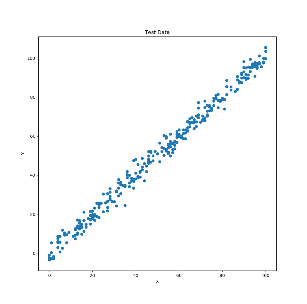
Test Data
The linear regression model fits a line through the data in the form $y=mx+b$ such that it tries to reduce the Sum of Squares Error (SSE). $$SSE= \sum_{i=0}^{n}(y_i-\hat y_i)^2$$ Where $y_i$ are the observed values (actual data points) and $\hat y_i$ are the predicted values (values from linear regression model $y=mx+b$). SSE quantifies the difference between the observed values and the predicted values. Other values that I will keep track of in the code are the Sum of Squares Regression (SSR), Sum of Squares Total (SSTO), and Coefficient of Determination ($R^2$). $$SSR= \sum_{i=0}^{n}(\hat y_i-\bar y)^2$$ $$SSTO= \sum_{i=0}^{n}(y_i-\bar y)^2$$ $$R^2= 1-\frac{SSE}{SSTO}$$ Where $\bar y$ is the mean of the observed data. SSR quantifies the difference between the predicted values and the mean of the observed values. SSTO quantifies the difference between the observed values and the mean of the observed values. An $R^2$ value of 1 means that the linear fit is perfect and goes through all the points since SSE=0 signifying that the predicted values are equal to the observed values $\hat y_i=y_i$. Creating a residual plot is also important as this provides information on whether or not the linear fit is a good fit. The residual plot should show no pattern and be centered around the x-axis in order to indicate that the linear fit is the correct fit. The residuals can be calculated with the following formula. $$e_i= y_i-\hat y_i$$
Code
Now that we know what we want to minimize in order to get the best fit line, we can apply the gradient descent algorithm to that function. Let the cost function of the linear regression model be the Mean of Squared Errors or MSE. We will use the gradient descent algorithm to find the minimum of the MSE in order to get the best fit line. $$MSE= \frac{1}{n} \sum_{i=0}^{n}(y_i-\hat y_i)^2$$ Applying the gradient descent algorithm to the MSE function we get (remember $\hat y_i=m_n x_i +b_n$): $$m_{n+1}= m_n - \alpha \nabla _{m_n} F$$ $$b_{n+1}= b_n - \alpha \nabla _{b_n} F$$ $$\nabla _{m_n} F= \frac{\partial F}{\partial m_n}=\frac{\partial MSE}{\partial m_n}=\frac{1}{n} \sum_{i=0}^{n}-2x_i \cdot (y_i-m_n x_i +b_n)$$ $$\nabla _{b_n} F= \frac{\partial F}{\partial b_n}=\frac{\partial MSE}{\partial b_n}=\frac{1}{n} \sum_{i=0}^{n}-2 \cdot (y_i-m_n x_i +b_n)$$ Note that we now have two variables m and b that we are updating at each iteration in order to minimize the MSE. We are not updating the x values at each iteration like in the previous example. Now that we know how to implement the gradient descent algorithm to a linear regression model, we can go ahead and write some Python code which I have broken down into sections below.
Lines 1-6 import the necessary libraries for this Python code. Line 9 imports the CSV file (which was downloaded from Kaggle) into a Pandas dataframe and lines 11-12 print out the first five rows of the CSV data. Lines 15 and 16 convert the data into numpy arrays in order to do calculations and operations with the data. Lines 18-34 set up the necessary variables and arrays for the gradient descent algorithm. Finally, lines 37-53 are the actual gradient descent algorithm that is minimizing the cost function MSE.
Lines 56-85 then create the animated plot of the linear regression model at each iteration after all the data has been calculated. The update() function on lines 73-79 updates the plot with the new linear regression model based off of the m and b value at that iteration. Lines 88-108 plot the errors and the coefficient of determination vs the iteration step. The starting point to plot the data was chosen when $R^2>0$ as this signifies that SSE < SSTO. This was done because at the beginning of the iterations, the linear regression model was significantly off causing $R^2 < 0$.
import pandas as pd
import numpy as np
import matplotlib.pyplot as plt
import matplotlib.animation as animation
from mpl_toolkits.mplot3d import Axes3D
from matplotlib import cm

# Importing csv data as Pandas dataframe
df_test = pd.read_csv(r'C:\Users\USERNAME\test.csv')

print('----------Test Data----------')
print(df_test.head())  # Printing first five rows of dataframe

# Converting data to array for later calculations
x_test = np.array(df_test['x'])
y_test = np.array(df_test['y'])

n = len(x_test)  # Number of samples in data

iter = 0  # Initial iteration counter
itersteps = 250  # Total number of iterations

# Initial guesses for linear regression model of y=mx+b and arrays to keep track of values over iterations
m = np.zeros(itersteps)
b = np.zeros(itersteps)
J = np.zeros(itersteps)
dJdm = np.zeros(itersteps)
dJdb = np.zeros(itersteps)
SSR = np.zeros(itersteps)
SSE = np.zeros(itersteps)
SSTO = np.zeros(itersteps)
R_sq = np.zeros(itersteps)

a = 1E-5  # Step size

# Gradient Descent implementation on the linear regression model
while iter < itersteps - 1:
    print('Iteration: ', iter)
    y_new = m[iter] * x_test + b[iter]

    J[iter] = 1 / n * np.sum((y_test - y_new) ** 2)  # Mean Squared Error

    dJdm[iter] = 1 / n * np.sum((y_test - y_new) * -2 * x_test)
    dJdb[iter] = 1 / n * np.sum((y_test - y_new) * -2)

    SSR[iter] = np.sum((y_new - np.mean(y_test)) ** 2)
    SSE[iter] = np.sum((y_test - y_new) ** 2)
    SSTO[iter] = np.sum((y_test - np.mean(y_test)) ** 2)
    R_sq[iter] = 1-SSE[iter]/SSTO[iter]

    m[iter + 1] = m[iter] - a * dJdm[iter]
    b[iter + 1] = b[iter] - a * dJdb[iter]
    iter += 1

# Data to create a smooth line for the linear regression model
x_min = min(x_test)
x_max = max(x_test)
x = np.linspace(x_min, x_max, n)
y = m[0] * x + b[0]

# Creating initial figure
fig1, ax, = plt.subplots(figsize=(10, 10))
ax.scatter(x_test, y_test)  # Initial scatter plot that does not get updated
line, = ax.plot(x, y, 'red')  # Initial linear fit
ax.set_xlabel('X')
ax.set_ylabel('Y')
t1 = ax.text(50, 25, 'Eqn: y=' + str(round(m[iter], 4)) + '*x+' + str(round(b[iter], 4)), fontsize=15) # Text displays y=mx+b on plot


# Function updates data for plot animation using animation.FuncAnimation() below
# The variable that is passed to this function from FuncAnimation is frames=itersteps-1
# This acquires the data at every iteration step
def update(iter):
    y = m[iter] * x + b[iter]  # The linear fit data at each iteration using m and b values at that iteration
    line.set_data(x, y)  # Updates linear fit data for plot
    t1.set_text('Eqn: y=' + str(round(m[iter], 4)) + '*x+' + str(round(b[iter], 4)))
    ax.set_title('Linear Regression with $R^2=$' + str(round(R_sq[iter], 4)) + ' iteration: ' + str(iter))
    ax.legend(bbox_to_anchor=(1, 1.2), fontsize='x-small')  # legend location and font
    return line, ax


# Animation function after all the variables at each iteration have been calculated
# Calls the function update and passes in the number of frames=itersteps-1 to get all the data at each iteration
ani = animation.FuncAnimation(fig1, update, frames=itersteps - 1, interval=10, blit=False, repeat_delay=100)
ani.save('lin_reg.mp4', fps=30, extra_args=['-vcodec', 'libx264'])  # Saves animation

# Figure of errors and coefficient of determination
R_sq0=np.where(R_sq>0) # Finds indices of where Rsq>0

fig2, ax2 = plt.subplots(figsize=(10, 10))

ax2.plot(np.arange(R_sq0[0][0], itersteps - 1), SSE[R_sq0[0][0]:-1], label='SSE', color='blue')
ax2.plot(np.arange(R_sq0[0][0], itersteps - 1), SSR[R_sq0[0][0]:-1], label='SSR', color='#0080ff')
ax2.plot(np.arange(R_sq0[0][0], itersteps - 1), SSTO[R_sq0[0][0]:-1], label='SSTO', color='#00c0ff')

ax2.set_title('Errors')
ax2.set_xlabel('Number of Iterations')
ax2.set_ylabel('Error', color='blue')
ax2.tick_params('y', colors='blue')

ax3 = ax2.twinx() # Second set of data on same x-axis
ax3.plot(np.arange(R_sq0[0][0], itersteps - 1), R_sq[R_sq0[0][0]:-1], color='red', label='$R^2$')
ax3.set_ylabel('Rsq', color='red')
ax3.tick_params('y', colors='red')

ax2.legend(bbox_to_anchor=(1, .60), fontsize='x-small')  # legend location and font size
ax3.legend(bbox_to_anchor=(1, .50), fontsize='x-small')  # legend location and font size
fig2.savefig('errors.png')  # saves figure
The two graphs generated in the above code can be seen below. In the animated linear regression plot, as the number of iterations progress, the linear fit improves as the gradient descent finds the values of m and b that minimize the MSE function. The SSE also decreases and $R^2$ increases as the number of iterations progress in the errors plot.
Linear Regression Gradient Descent
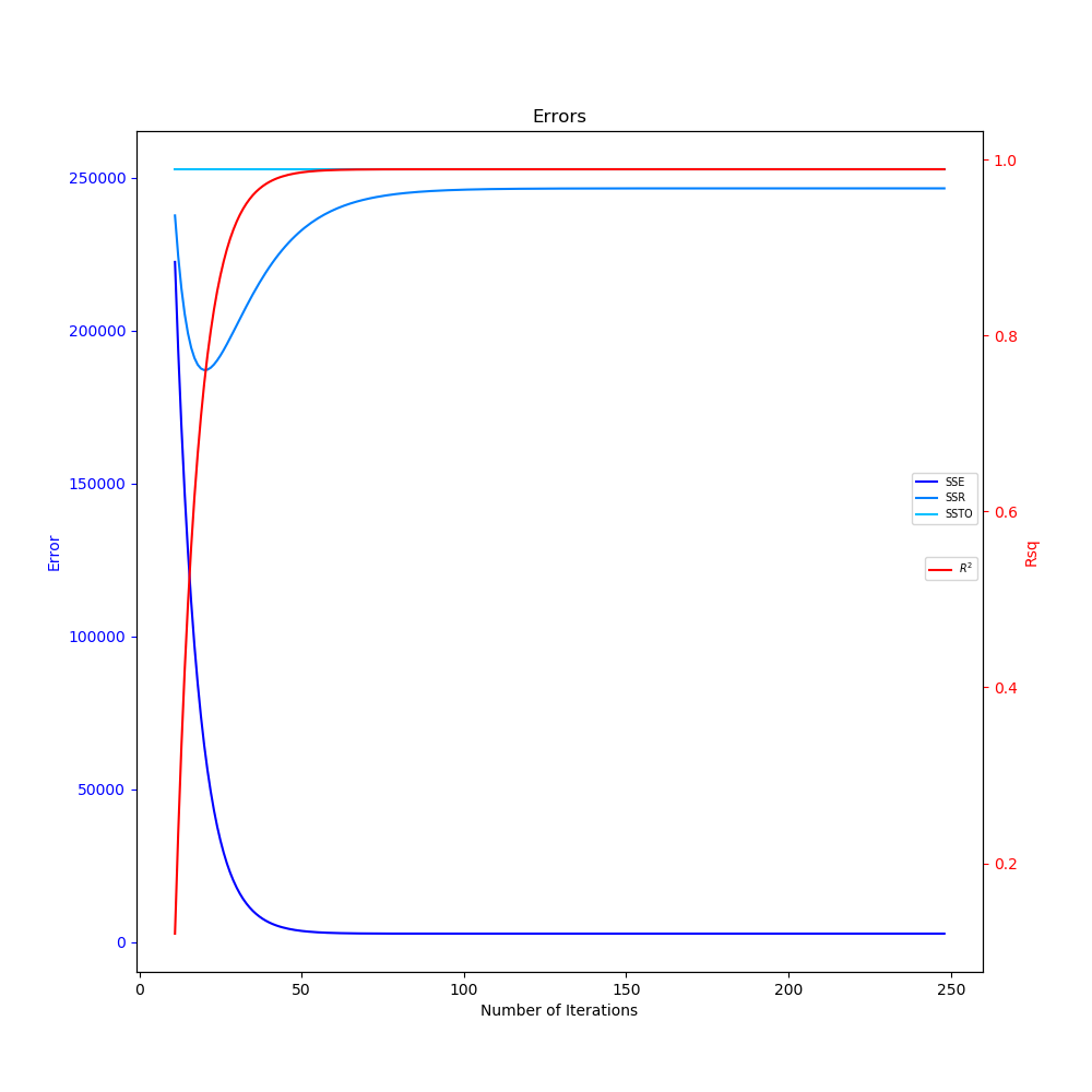
Errors and Coefficient of Determination
I was curious to see what the 3D Surface Plot of the MSE function would look like with different combinations of m and b and what values m and b minimize the MSE function. Below is the code that creates such plot.
Lines 111-115 set up the grid for the different values of m and b and the matrix that will contain the values of the MSE. It is important to refine the grid in lines 111-113 as the m and b values that minimize the MSE might be in a section that the grid does not cover or the grid is not fine enough to capture those m and b values. Lines 118-122 then calculate the MSE matrix for all the different combinations of m and b.
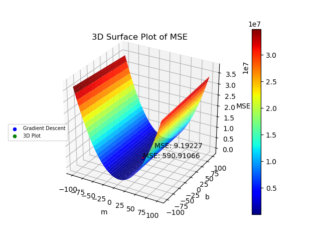
Lines 125-145 create the 3D surface plot of the MSE and plot the minimum values of MSE for both the Gradient Descent method and the 3D Plot. Line 130 plots the journey of the MSE for the Gradient Descent method as the number of iterations progress. Lines 132 and 140 plot the final minimum MSE for both methods. Lines 151-186 calculate and plot the linear regression models on the original data using both the Gradient Descent Method and the 3D plot. Lines 189-200 plot the residuals for both methods. Finally, lines 203-217 plot the contour of the 3D surface plot to better depict the MSE values for both methods.
# Creating mesh for 3D Surface Plot of MSE
mm = np.linspace(-10, 10, 1000)
bb = np.linspace(-10, 10, 1000)
mmm, bbb = np.meshgrid(mm, bb)

JJ = np.zeros([len(mm), len(bb)])

# Calculating values of MSE for different combinations of m and b
for i in range(len(mm)):
    for j in range(len(bb)):
        print('i: ',i, 'j: ', j)
        yy = mmm[i, j] * x_test + bbb[i, j]
        JJ[i, j] = 1 / n * np.sum((y_test - yy) ** 2)

# 3D Surface Plot
fig3 = plt.figure()
ax4 = fig3.gca(projection='3d')
surf = ax4.plot_surface(mmm, bbb, JJ, cmap=plt.cm.jet)
fig3.colorbar(surf)

ax4.plot(m[:-1], b[:-1], J[:-1], 'red')
ax4.scatter(m[-2], b[-2], J[-2], c='b', marker="o",label='Gradient Descent')
ax4.text(m[-2], b[-2], J[-2], '%s' % ('MSE: '+str(round(J[-2],5))), color='k')
ax4.set_xlabel('m')
ax4.set_ylabel('b')
ax4.set_zlabel('MSE')
ax4.set_title('3D Surface Plot of MSE')

# Acquiring and plotting minimum value of MSE
i_min, j_min = np.unravel_index(JJ.argmin(), JJ.shape)
ax4.scatter(mmm[i_min, j_min], bbb[i_min, j_min], np.min(JJ), c='g', marker="o",label='3D Plot')
ax4.text(mmm[i_min, j_min], bbb[i_min, j_min], np.min(JJ), '%s' % ('MSE: '+str(round(np.min(JJ),5))), color='k')

ax4.legend(bbox_to_anchor=(0.15, .50), fontsize='x-small')

fig3.savefig('MSE_3D.png')  # saves figure


# Calculating linear fit and errors for both methods
# Gradient Descent
y = m[-1] * x_test + b[-1] # Predicted Values
y2 = m[-1] * x + b[-1] # Linear fit
SSR1 = np.sum((y - np.mean(y_test)) ** 2)
SSE1 = np.sum((y_test - y) ** 2)
SSTO1 = np.sum((y_test - np.mean(y_test)) ** 2)
R_sq1 = 1-SSE1/SSTO1

# 3D Plot
yyy = mmm[i_min, j_min] * x_test + bbb[i_min, j_min] # Predicted Values
yyy2 = mmm[i_min, j_min] * x + bbb[i_min, j_min] # Linear fit
SSR2 = np.sum((yyy - np.mean(y_test)) ** 2)
SSE2 = np.sum((y_test - yyy) ** 2)
SSTO2 = np.sum((y_test - np.mean(y_test)) ** 2)
R_sq2 = 1-SSE2/SSTO2


# Printing Min MSE, m, and b for both methods
print('Gradient Descent Min MSE: ', J[-2])
print('Gradient Descent m: ', m[-2], ' and b: ', b[-2])
print('Gradient Descent $R^2$: ', R_sq1)
print('3D Plot Min MSE: ', np.min(JJ))
print('3D Plot m: ', mmm[i_min, j_min], ' and b: ', bbb[i_min, j_min])
print('3D Plot $R^2$: ', R_sq2)


# Linear fit for both methods on scatter plot
fig4, ax5 = plt.subplots(figsize=(10, 10))
ax5.scatter(x_test, y_test)  # initial data that does not get updated
ax5.plot(x, y2, 'blue', label='Gradient Descent: y=' + str(round(m[-1], 5)) + '*x+' + str(round(b[-1], 5)) + ' $R^2=$' + str(round(R_sq1, 5)))  # initial linear fit
ax5.plot(x, yyy2, 'green', label='3D Plot: y=' + str(round(mmm[i_min, j_min], 5)) + '*x+' + str(round(bbb[i_min, j_min], 5)) + ' $R^2=$' + str(round(R_sq2, 5)))  # initial linear fit
ax5.set_title('Linear Regression')
ax5.set_xlabel('X')
ax5.set_ylabel('Y')
ax5.legend()

fig4.savefig('lin_reg_both.png')  # saves figure

# Residual plot for both methods
e1=y_test-y
e2=y_test-yyy

fig5, ax6 = plt.subplots(figsize=(10, 10))
ax6.scatter(x_test, e1, c='blue', label='Gradient Descent: y=' + str(round(m[-1], 5)) + '*x+' + str(round(b[-1], 5)) + ' $R^2=$' + str(round(R_sq1, 5)))  # initial linear fit
ax6.scatter(x_test, e2, c='green', label='3D Plot: y=' + str(round(mmm[i_min, j_min], 5)) + '*x+' + str(round(bbb[i_min, j_min], 5)) + ' $R^2=$' + str(round(R_sq2, 5)))  # initial linear fit
ax6.set_title('Residuals')
ax6.set_xlabel('X')
ax6.set_ylabel('Residual')
ax6.legend()

fig5.savefig('res_both.png')  # saves figure

# Contour plot of 3D plot
fig6, ax7 = plt.subplots(figsize=(10, 10))
ax7.contour(mmm, bbb, JJ, 100, cmap=plt.cm.jet);
ax7.plot(m[:-1], b[:-1], 'red')
ax7.scatter(m[-2], b[-2], c='b', marker="o",label='Gradient Descent: y=' + str(round(m[-1], 5)) + '*x+' + str(round(b[-1], 5)) + ' $R^2=$' + str(round(R_sq1, 5)))
ax7.text(m[-2], b[-2], '%s' % ('MSE: '+str(round(J[-2],5))), color='k')
ax7.scatter(mmm[i_min, j_min], bbb[i_min, j_min], c='g', marker="o",label='3D Plot: y=' + str(round(mmm[i_min, j_min], 5)) + '*x+' + str(round(bbb[i_min, j_min], 5)) + ' $R^2=$' + str(round(R_sq2, 5)))
ax7.text(mmm[i_min, j_min], bbb[i_min, j_min], '%s' % ('MSE: '+str(round(np.min(JJ),5))), color='k')
ax7.set_xlabel('m')
ax7.set_ylabel('b')
ax7.set_title('Contour Plot of MSE')
ax7.legend()

fig6.savefig('contour.png')  # saves figure

plt.show()  # Show all plots
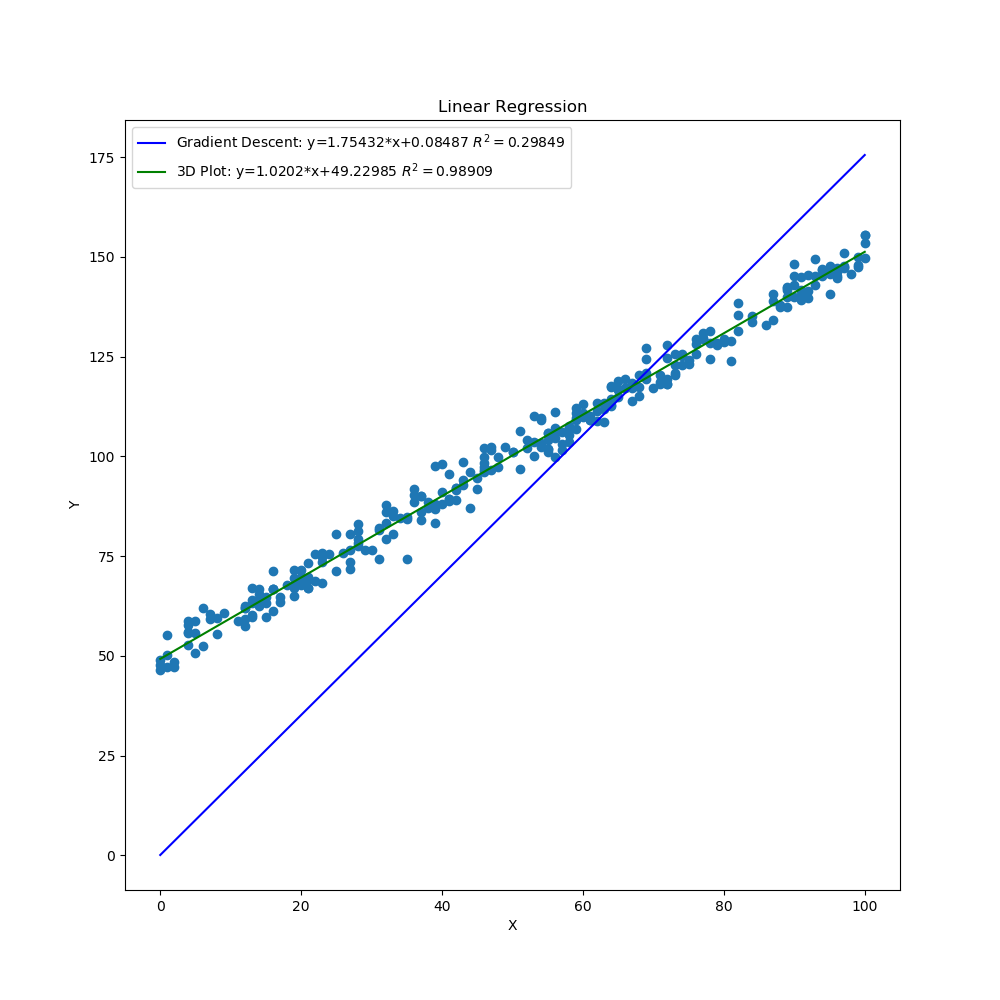
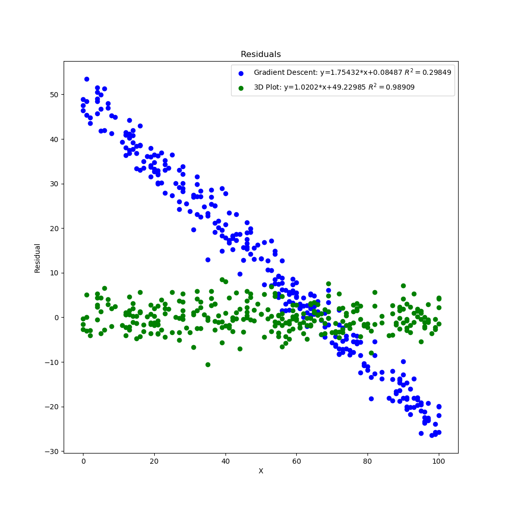
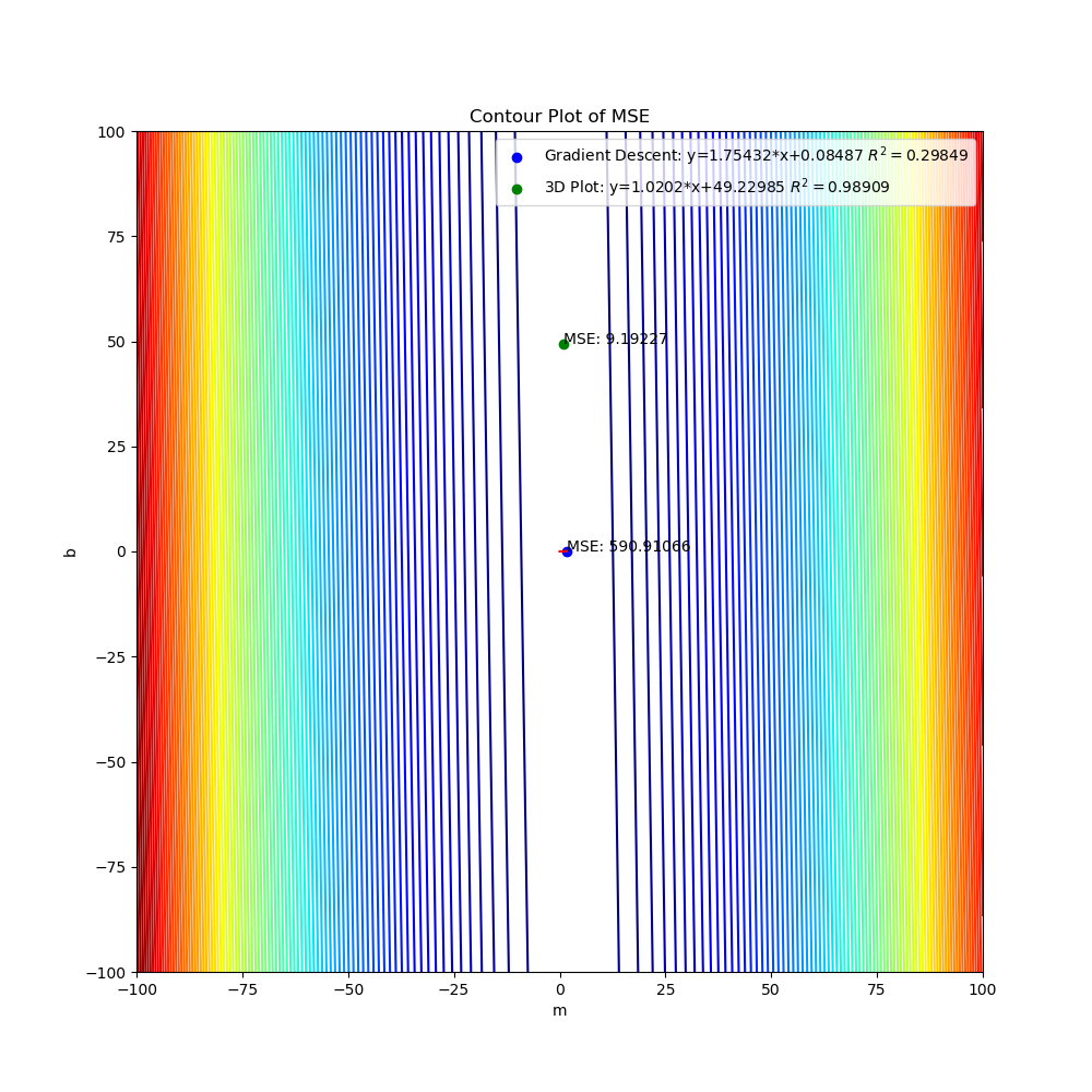
The graphs created by the code above can be seen below. The 3D surface plot depicts the different values of MSE one would get depending on the different combinations of m and b. The final MSE for both methods are also plotted on the 3D graph. The linear fit for both methods are very close to one another but the 3D Plot is a bit better due to the fine grid and location of grid (if either one of those were off, then the linear regression model would be off too since m and b would not be accurate). Also, the step size of the gradient descent and the gradual slope of the function can cause the gradient descent to take longer to descend to a minima as will be seen in the section below. The residual plot for both methods indicate that a linear fit is a good fit since the residuals show no apparent pattern. The contour plot illustrates the minimum MSE values for both methods in a clearer manner. Both $R^2$ and MSE values are very close to one another. The $R^2$ values are close to 1 signifying a good liner fit.
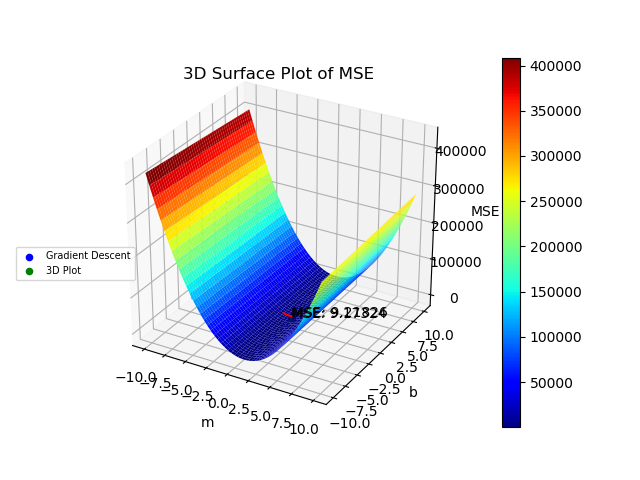
MSE 3D
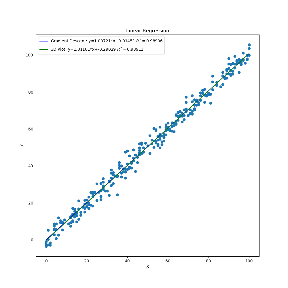
Linear Regression Both Methods
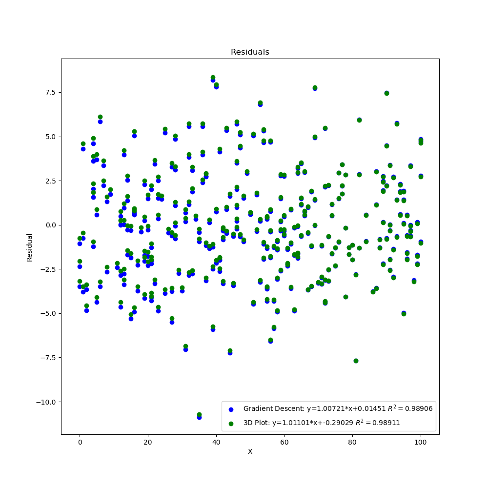
Residual Plot Both Methods
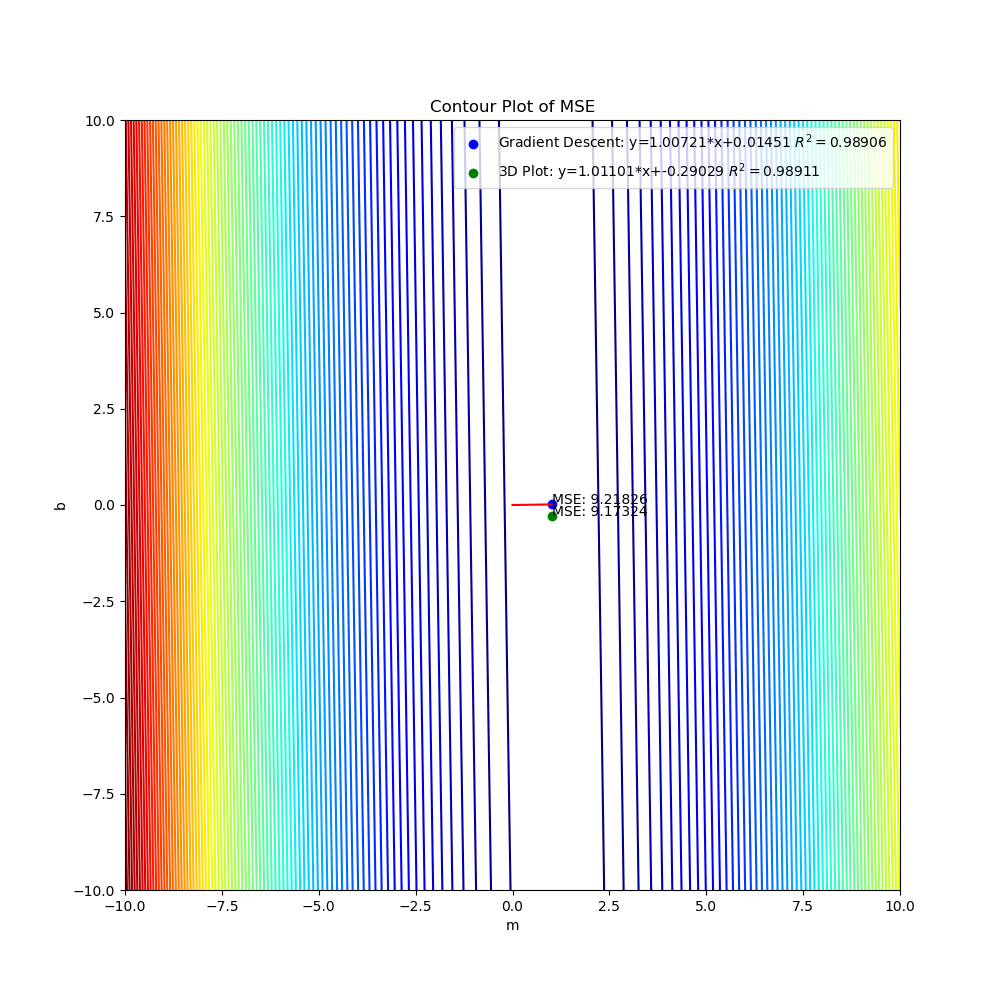
Contour Plot
As mentioned before, the initial guess of the gradient descent algorithm can have a great influence on finding the minimum. Here, I updated line 15 to shift all the y data points by 50 but kept the initial point the same on lines 24-25. I also updated the grid in lines 111-112 (this will take a lot longer since each axis now has 5000 points instead of 1000) to better capture the values of m and b that will give the minimum MSE with a good $R^2$ value. After running the code, the gradient descent algorithm does not do a very good job of finding the minimum due to the initial guess. The slope is gradual so the process to a better minimum would require a lot more iterations. Here the $R^2$ and MSE values are very different from one another with one linear fit being a lot better than the other.
y_test = np.array(df_test['y'])+50
mm = np.linspace(-100, 100, 5000)
bb = np.linspace(-100, 100, 5000)
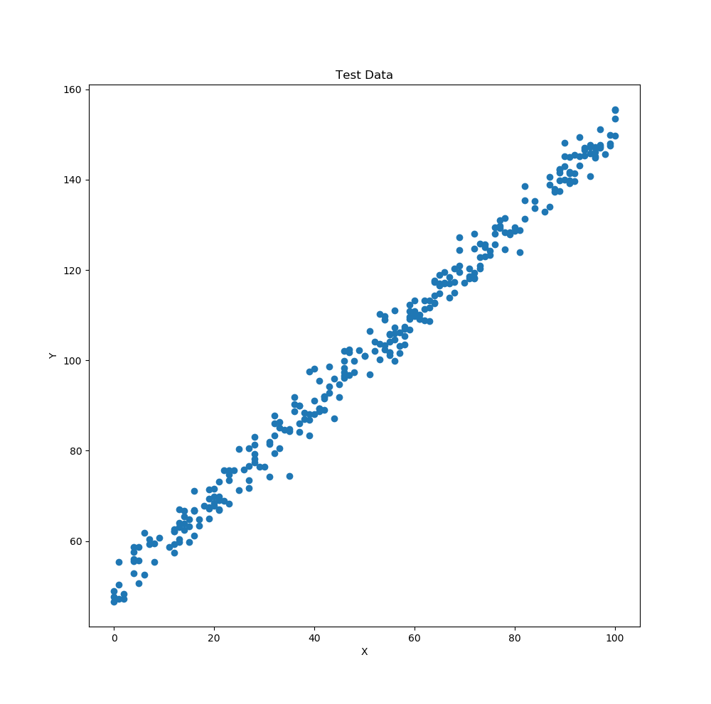
Test Data Shifted Y
Linear Regression Gradient Descent Shifted Y
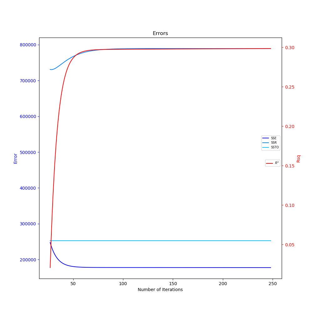
Errors and Coefficient of Determination Shifted Y
MSE 3D Shifted Y
Linear Regression Both Methods Shifted Y
Residual Plot Both Methods Shifted Y
Contour Plot Shifted Y